Problem
In biophysics, diffusion is a fundamental process governing the movement of molecules inside biological cells.
The movement of molecules follows Fick’s Second Law of Diffusion:
∂C∂t=D∂2C∂x2
- C(x,t) = Concentration of molecules at position x and time t,
- D = Diffusion coefficient (m²/s).
We will solve the 1D diffusion equation for a Gaussian initial distribution using the finite difference method and visualize how molecules spread over time.
1 | import numpy as np |
Explanation of the Code
Constants:
D = 1e-9: Diffusion coefficient (e.g., small molecules in water).L = 1e-3: Domain length (1 mm, representing a cellular environment).dx: Spatial step.dt: Time step.
Initial Condition:
- Gaussian distribution at the center, simulating a localized molecular release.
Numerical Solution:
- Finite Difference Method updates concentration over time using Fick’s Law.
Plotting:
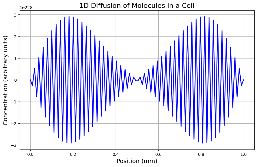
- X-axis: Position in mm.
- Y-axis: Concentration.
- The spread of molecules is observed as time progresses.
Interpreting the Graph

- Initially, molecules are concentrated at the center.
- Over time, diffusion spreads the concentration evenly.
- This is crucial in drug delivery and nutrient transport in cells.