
非線形/多変数方程式
以下のような関数を考えてみましょう。
この関数は非線形で多変数の方程式であり、解析的な解法は難しいとされています。
f(x,y)=sin(√x2+y2)−x2−y3
この方程式の解を求め、結果を3Dグラフ化します。
1 | import numpy as np |
この例では、Scipyのfsolveを使用して非線形方程式の数値解を求め、得られた解を3Dグラフ上にプロットしています。
[実行結果]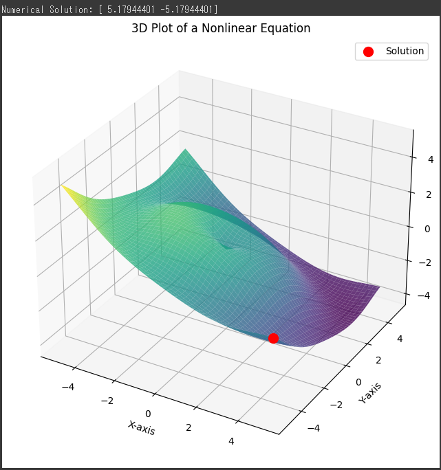
ソースコード解説
以下に、ソースコードの詳細な説明を示します。
1. ライブラリのインポート
1 | import numpy as np |
必要なライブラリをインポートしています。
numpyは数値計算を行うために使用されます。matplotlib.pyplotはグラフ描画のために使用されます。scipy.optimize.fsolveは非線形方程式の数値解を求めるために使用されます。mpl_toolkits.mplot3dは3Dグラフ描画のために使用されます。
2. 非線形方程式の定義
1 | def equation(vars): |
equation関数では、2つの変数(x)と(y)に対する非線形方程式が定義されています。
この例では、[sin(√x2+y2)−x2−y3]および(x+y)という2つの方程式が組み合わさっています。
3. 初期値の設定
1 | initial_guess = [1, 1] |
非線形方程式の数値解を求める際に使用する初期の予測値を設定しています。
4. 非線形方程式の数値解を求める
1 | solution = fsolve(equation, initial_guess) |
fsolve関数を用いて、equation関数に定義された非線形方程式の数値解を求めます。
解は solution に格納され、その値が表示されます。
5. 3Dグラフの描画
1 | fig = plt.figure(figsize=(10, 8)) |
Matplotlibを使用して3Dグラフを描画するための準備を行います。
6. 関数の値を計算してプロット
1 | x_vals = np.linspace(-5, 5, 100) |
指定された範囲内の(x)と(y)の値を生成し、それに対応する関数の値を計算して3Dプロットします。
7. 解の点をプロット
1 | ax.scatter(solution[0], solution[1], np.sin(np.sqrt(solution[0]**2 + solution[1]**2)) - solution[0]/2 - solution[1]/3, color='red', marker='o', s=100, label='Solution') |
先ほど求めた数値解を3Dプロットに赤い点として追加します。
8. グラフの設定
1 | ax.set_title('3D Plot of a Nonlinear Equation') |
グラフのタイトルや軸のラベルを設定し、凡例を表示します。
9. グラフの表示
1 | plt.show() |
最後に、Matplotlibを使用して描画したグラフを表示します。
これにより、非線形方程式の数値解とそのグラフが視覚的に確認できます。
結果解説
[実行結果]
表示されたNumerical Solution ([5.17944401, -5.17944401]) は、非線形方程式
f(x,y)=sin(√x2+y2)−x2−y3
の数値解です。
この解は、関数(f(x,y))がゼロになる点を表しています。
具体的には、(x=5.17944401)および(y=−5.17944401)で、この点で方程式が満たされています。
グラフの3Dプロットでは、関数(f(x,y))の曲面を表示しています。
この曲面上で、赤い点が数値解を表しています。
赤い点が曲面と交差する点が方程式の解であり、その座標が表示された数値解と一致しています。
数値解を求めるプロセスは、初期の予測値(initial_guess)から始まり、Scipyのfsolveが方程式に対して最適な値を見つけるために反復的な手法を使用します。
このプロセスは非線形方程式に対して一般的に使用され、数値的に解を見つけることができます。
この例では、与えられた非線形方程式を解くためにScipyを利用し、得られた数値解を3Dグラフ上に視覚化しました。