多項式関数
複雑な数式として、例えば次のような多項式関数を考えてみましょう。
$$
f(x, y) = \sin(x^2 + y^2) \cdot \cos(xy)
$$
このような関数を3Dグラフで表現することができます。
以下は、この関数のグラフをPythonでプロットする例です。
1 | import numpy as np |
これにより、関数$ f(x, y) = \sin(x^2 + y^2) \cdot \cos(xy) $の3Dグラフが生成されます。
[実行結果]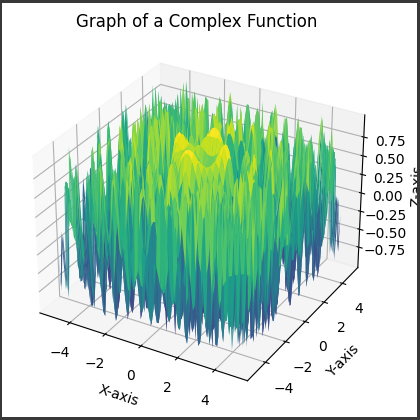
数式を変更して他の複雑な関数をプロットすることもできます。
ソースコード解説
以下に、コードの各部分を詳しく説明します。
1. numpyライブラリの導入:
1 | import numpy as np |
数値計算に使用されるNumPyライブラリを導入しています。
2. matplotlib.pyplotおよびmpl_toolkits.mplot3dの導入:
1 | import matplotlib.pyplot as plt |
Matplotlibのpyplotモジュールと3DプロットのためのAxes3Dを導入しています。
3. データの生成:
1 | x = np.linspace(-5, 5, 100) |
xとyはそれぞれ$-5$から$5$までの範囲で等間隔に$100$点生成されます。np.meshgridを使用して2つの1次元配列をグリッドデータに変換し、zは複雑な関数の値が計算されます。
この場合、z = sin(x**2 + y**2) * cos(x * y) です。
4. 3Dプロットの作成:
1 | fig = plt.figure() |
MatplotlibのFigureオブジェクトと3Dサブプロットを作成します。
5. 3Dサーフェスプロット:
1 | ax.plot_surface(x, y, z, cmap='viridis') |
ax.plot_surfaceを使用して、x、y、およびzで表される3Dサーフェスプロットを作成します。cmapパラメータはカラーマップを指定しています。
ここでは’viridis’を使用しています。
6. 軸ラベルとタイトルの設定:
1 | ax.set_xlabel('X-axis') |
X軸、Y軸、およびZ軸のラベルを設定し、グラフにタイトルを追加します。
7. グラフの表示:
1 | plt.show() |
最後にplt.show()を呼び出して、グラフを表示します。
このコードによって生成されるグラフは、3Dサーフェスプロットで表される関数の形状を示しています。
関数は $x$, $y$ の二乗の和と $x$ と$ y $の積に依存しており、$sin$ および$ cos $関数を組み合わせています。
グラフの形状や色合いは、この複雑な関数の値に基づいています。