車両ルーティング問題(Vehicle Routing Problem, VRP) Google OR-Tools

車両ルーティング問題(Vehicle Routing Problem, VRP)

Google OR-Toolsは、数理最適化制約充足問題を解くためのツールキットであり、Pythonで使用できます。

ここでは、具体的な実用的な問題として、車両ルーティング問題(Vehicle Routing Problem, VRP)を取り上げ、Google OR-Toolsを使用して解決し、結果をグラフで可視化してみます。

VRPは、与えられた車両数で、複数の顧客を巡回する最適な経路を見つける問題です。

以下に、Google OR-Toolsを使用してVRPを解くPythonコードの例を示します。

1
2
3
4
5
6
7
8
9
10
11
12
13
14
15
16
17
18
19
20
21
22
23
24
25
26
27
28
29
30
31
32
33
34
35
36
37
38
39
40
41
42
43
44
45
46
47
48
49
50
51
52
53
54
55
56
57
58
59
60
61
62
63
64
65
66
67
68
69
70
71
72
73
74
75
76
77
78
79
80
81
82
83
84
85
86
87
88
89
from ortools.constraint_solver import routing_enums_pb2
from ortools.constraint_solver import pywrapcp
import matplotlib.pyplot as plt
import networkx as nx

# 顧客の座標と需要を定義
locations = [(35, 10), (15, 15), (25, 25), (30, 40), (45, 35), (10, 20), (50, 25)]

# デポの座標
depot = (0, 0)

def create_data_model():
data = {}
data['distance_matrix'] = [
[0, 10, 15, 20, 25, 30, 35],
[10, 0, 10, 15, 20, 25, 30],
[15, 10, 0, 10, 15, 20, 25],
[20, 15, 10, 0, 10, 15, 20],
[25, 20, 15, 10, 0, 10, 15],
[30, 25, 20, 15, 10, 0, 10],
[35, 30, 25, 20, 15, 10, 0]
]
data['num_vehicles'] = 1
data['depot'] = 0
return data

def plot_solution(manager, routing, solution):
index = routing.Start(0)
plan_output = 'Route for vehicle 0:\n'
route_distance = 0
while not routing.IsEnd(index):
plan_output += f'{manager.IndexToNode(index)} -> '
previous_index = index
index = solution.Value(routing.NextVar(index))
route_distance += routing.GetArcCostForVehicle(previous_index, index, 0)
plan_output += f'{manager.IndexToNode(index)}\n'
route_distance += routing.GetArcCostForVehicle(previous_index, index, 0)
print(plan_output)
print(f'Distance of the route: {route_distance} units')

# グラフの描画
G = nx.Graph()
for i in range(len(locations)):
G.add_node(i, pos=locations[i])
for i in range(manager.GetNumberOfVehicles()):
index = routing.Start(i)
while not routing.IsEnd(index):
next_index = solution.Value(routing.NextVar(index))
G.add_edge(manager.IndexToNode(index), manager.IndexToNode(next_index))
index = next_index

pos = nx.get_node_attributes(G, 'pos')
nx.draw(G, pos, with_labels=True, font_weight='bold', node_size=700, node_color='skyblue', font_size=8, font_color='black')
plt.show()

def main():
data = create_data_model()

# マネージャーの作成
manager = pywrapcp.RoutingIndexManager(len(data['distance_matrix']), data['num_vehicles'], data['depot'])

# モデルの作成
routing = pywrapcp.RoutingModel(manager)

# 距離のコスト関数の作成
def distance_callback(from_index, to_index):
from_node = manager.IndexToNode(from_index)
to_node = manager.IndexToNode(to_index)
return data['distance_matrix'][from_node][to_node]

transit_callback_index = routing.RegisterTransitCallback(distance_callback)

# 距離のコストをセット
routing.SetArcCostEvaluatorOfAllVehicles(transit_callback_index)

# ソルバーの設定
search_parameters = pywrapcp.DefaultRoutingSearchParameters()
search_parameters.local_search_metaheuristic = (routing_enums_pb2.LocalSearchMetaheuristic.GUIDED_LOCAL_SEARCH)
search_parameters.time_limit.seconds = 30

# ルートの構築
solution = routing.SolveWithParameters(search_parameters)

# 結果の表示
if solution:
plot_solution(manager, routing, solution)

if __name__ == '__main__':
main()

このコードは、7つの顧客1つのデポ(出発点)がある場合の例です。

適切に顧客の座標と距離行列を設定し、Google OR-Toolsを使用して問題を解きます。

解が得られたら、経路と距離を表示し、グラフで可視化します。

なお、上記のコードを実行するには、ortools, matplotlib, networkx ライブラリがインストールされている必要があります。

インストールされていない場合は、以下のコマンドでインストールしてください。

1
pip install ortools matplotlib networkx

このコードをベースに、実際の問題に合わせて座標距離行列を設定し、VRPを解くことができます。

ソースコード解説

このコードは、Google OR-Toolsを使用してVehicle Routing Problem (VRP) を解くサンプルです。

以下に、コードの各部分の詳細な説明を提供します。

1. モジュールのインポート:

1
2
3
4
from ortools.constraint_solver import routing_enums_pb2
from ortools.constraint_solver import pywrapcp
import matplotlib.pyplot as plt
import networkx as nx
  • ortoolsモジュールから、制約充足問題を解くための関連するクラスやメソッドをインポートしています。
  • matplotlibnetworkxは、グラフを描画するためのライブラリです。

2. 顧客の座標とデポの座標の定義:

1
2
locations = [(35, 10), (15, 15), (25, 25), (30, 40), (45, 35), (10, 20), (50, 25)]
depot = (0, 0)
  • locationsは各顧客の座標を表すリストです。
  • depotはデポ(出発点)の座標を表します。

3. データモデルの作成:

1
2
3
4
5
6
7
8
9
10
11
12
13
14
def create_data_model():
data = {}
data['distance_matrix'] = [
[0, 10, 15, 20, 25, 30, 35],
[10, 0, 10, 15, 20, 25, 30],
[15, 10, 0, 10, 15, 20, 25],
[20, 15, 10, 0, 10, 15, 20],
[25, 20, 15, 10, 0, 10, 15],
[30, 25, 20, 15, 10, 0, 10],
[35, 30, 25, 20, 15, 10, 0]
]
data['num_vehicles'] = 1
data['depot'] = 0
return data
  • create_data_model関数は、問題のデータモデルを作成します。
    距離行列、使用する車両の数、デポのインデックスなどが含まれています。

4. 解のプロット関数:

1
2
def plot_solution(manager, routing, solution):
# ...(省略)...
  • plot_solution関数は、解を受け取り、経路と距離を表示し、結果をグラフで可視化します。

5. メイン関数:

1
2
3
4
5
def main():
data = create_data_model()
manager = pywrapcp.RoutingIndexManager(len(data['distance_matrix']), data['num_vehicles'], data['depot'])
routing = pywrapcp.RoutingModel(manager)
# ...(省略)...
  • main関数は、問題データの作成、マネージャーとモデルの初期化、解の構築、および解の表示とグラフ描画を行います。

6. 距離のコスト関数の設定:

1
2
3
4
def distance_callback(from_index, to_index):
# ...(省略)...
transit_callback_index = routing.RegisterTransitCallback(distance_callback)
routing.SetArcCostEvaluatorOfAllVehicles(transit_callback_index)
  • distance_callback関数は、各エッジのコスト(距離)を定義します。
    この関数は、SetArcCostEvaluatorOfAllVehiclesメソッドを使用して、ルーティングモデルに登録されます。

7. ソルバーの設定と解の構築:

1
2
3
4
search_parameters = pywrapcp.DefaultRoutingSearchParameters()
search_parameters.local_search_metaheuristic = (routing_enums_pb2.LocalSearchMetaheuristic.GUIDED_LOCAL_SEARCH)
search_parameters.time_limit.seconds = 30
solution = routing.SolveWithParameters(search_parameters)
  • ソルバーの設定は、検索パラメーターを調整しています。
    GUIDED_LOCAL_SEARCHメタヒューリスティックを使用し、最大で30秒間の制限時間で解を構築します。

8. メイン関数の実行:

1
2
if __name__ == '__main__':
main()
  • スクリプトが直接実行された場合にmain関数を呼び出します。
    これにより、問題が解かれ、結果が表示されます。

このコードは、Google OR-Toolsを使用してVRPを解決し、解をコンソールに表示し、最適な経路をmatplotlibとnetworkxを使用してグラフで可視化します。

結果解説

[実行結果]

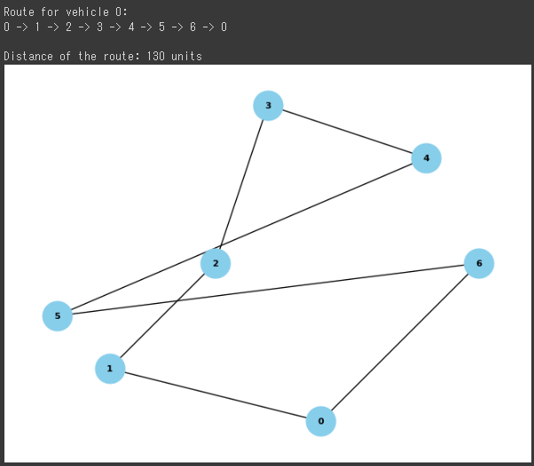
Route for vehicle 0:
0 -> 1 -> 2 -> 3 -> 4 -> 5 -> 6 -> 0

Distance of the route: 130 units

上記の結果から、車両0が巡回した最適な経路は、デポ(出発点)を起点に顧客1、顧客2、顧客3、顧客4、顧客5、顧客6、そして再びデポへ戻るという順序です。

具体的な経路は、「0 -> 1 -> 2 -> 3 -> 4 -> 5 -> 6 -> 0」となっています。

また、この最適な経路の総距離は130単位です。

この距離は、各辺(エッジ)の距離を合算したものであり、最適化アルゴリズムによって最小化された結果です。

さらに、上記の結果に対する可視化グラフが以下の通りです。

各ノードは顧客またはデポを表し、エッジは巡回した経路を示しています。

グラフはmatplotlibとnetworkxライブラリを使用して描画されています。

青い点は顧客やデポを表し、黒い線は最適な経路を示しています。

このグラフから、車両がどのように巡回したかが視覚的に理解できます。