ResNet (Resiidual Network) で画像分類

ResNet (Resiidual Network) で画像分類を行います。

ResNetでは残差ブロックというショートカット構造があることが特徴です。
畳み込み層にショートカットコネクション(迂回ルート)を追加し、畳み込み層で学習が不要になった場合迂回を行いより深い層の学習ができるようになります。

まずGoogle Colaboratoryのランタイムのハードウェアアクセラレータを「TPU」に設定します。
ハードウェアアクセラレータの設定

次にtensorflowのバージョンを1.13.1にします。

1
2
!pip uninstall tensorflow -y
!pip install tensorflow==1.13.1

インストール後にランタイムをリスタートする必要があります。


ResNetで必要なパッケージをインポートします。

1
2
3
4
5
6
7
8
9
10
11
12
# パッケージのインポート
from tensorflow.keras.datasets import cifar10
from tensorflow.keras.callbacks import LearningRateScheduler
from tensorflow.keras.layers import Activation, Add, BatchNormalization, Conv2D, Dense, GlobalAveragePooling2D, Input
from tensorflow.keras.models import Model
from tensorflow.keras.optimizers import SGD
from tensorflow.keras.preprocessing.image import ImageDataGenerator
from tensorflow.keras.regularizers import l2
from tensorflow.keras.utils import to_categorical
import numpy as np
import matplotlib.pyplot as plt
%matplotlib inline

データセットの準備を行います。

データセットの配列は下記のようになります。

配列 説明
train_images 訓練画像の配列
train_labels 訓練ラベルの配列
test_images テスト画像の配列
test_labels テストラベルの配列
1
2
# データセットの準備
(train_images, train_labels), (test_images, test_labels) = cifar10.load_data()

実行結果1

データセットのシェイプを確認します、

1
2
3
4
5
# データセットのシェイプの確認
print(train_images.shape)
print(train_labels.shape)
print(test_images.shape)
print(test_labels.shape)

実行結果2

訓練データと訓練ラベルは50000件、テスト画像とテストラベルは10000件です。
画像サイズは32×32×3です。RGB画像のため画像サイズ(32×32)×3となります。


先頭10件の訓練画像を確認します。

1
2
3
4
5
# データセットの画像の確認
for i in range(10):
plt.subplot(2, 5, i+1)
plt.imshow(train_images[i])
plt.show()

実行結果3

先頭10件の訓練ラベルの確認を行います。

1
2
# データセットのラベルの確認
print(train_labels[0:10])

実行結果4

ラベルの意味は下記の通りです。

ID 説明
0 airplane(飛行機)
1 automobile(自動車)
2 bird(鳥)
3 cat(猫)
4 deer(鹿)
5 dog(犬)
6 frog(カエル)
7 horse(馬)
8 ship(船)
9 truck(トラック)

データセットの前処理と確認を行います。

訓練ラベルとテストラベルのone-hot表現への変換を行います。

1
2
3
4
5
6
7
8
9
10
11
# データセットの前処理
train_images = train_images
train_labels = to_categorical(train_labels)
test_images = test_images
test_labels = to_categorical(test_labels)

# データセットの前処理後のシェイプの確認
print(train_images.shape)
print(train_labels.shape)
print(test_images.shape)
print(test_labels.shape)

実行結果5

畳み込み層の生成を行います。

Conv2Dのコンストラクタの引数は次の通りです。

引数 データ型 説明
filters int カーネル数
kernel_size int or tuple カーネルサイズ
strides int or tuple ストライド
padding str パディングで入力と同じサイズに戻すときはsame、戻さないときはvalid
user_bias boot バイアスを加えるかどうか
kernel_initializer str カーネルの重み行列の初期値。he_normalは正規分布による初期化
kernel_regularizer Regularizer kernelの重みに適用させる正則化。l2はL2正則化を利用
1
2
3
4
# 畳み込み層の生成
def conv(filters, kernel_size, strides=1):
return Conv2D(filters, kernel_size, strides=strides, padding='same', use_bias=False,
kernel_initializer='he_normal', kernel_regularizer=l2(0.0001))

残差ブロックAを生成します。

1
2
3
4
5
6
7
8
9
10
11
12
13
14
15
16
17
18
19
20
21
22
23
24
25
26
# 残差ブロックAの生成
def first_residual_unit(filters, strides):
def f(x):
# →BN→ReLU
x = BatchNormalization()(x)
b = Activation('relu')(x)

# 畳み込み層→BN→ReLU
x = conv(filters // 4, 1, strides)(b)
x = BatchNormalization()(x)
x = Activation('relu')(x)

# 畳み込み層→BN→ReLU
x = conv(filters // 4, 3)(x)
x = BatchNormalization()(x)
x = Activation('relu')(x)

# 畳み込み層→
x = conv(filters, 1)(x)

# ショートカットのシェイプサイズを調整
sc = conv(filters, 1, strides)(b)

# Add
return Add()([x, sc])
return f

残差ブロックBを生成します。

1
2
3
4
5
6
7
8
9
10
11
12
13
14
15
16
17
18
19
20
21
22
23
24
25
# 残差ブロックBの生成
def residual_unit(filters):
def f(x):
sc = x

# →BN→ReLU
x = BatchNormalization()(x)
x = Activation('relu')(x)

# 畳み込み層→BN→ReLU
x = conv(filters // 4, 1)(x)
x = BatchNormalization()(x)
x = Activation('relu')(x)

# 畳み込み層→BN→ReLU
x = conv(filters // 4, 3)(x)
x = BatchNormalization()(x)
x = Activation('relu')(x)

# 畳み込み層→
x = conv(filters, 1)(x)

# Add
return Add()([x, sc])
return f

残差ブロックAと残差ブロックB x 17を生成します。

1
2
3
4
5
6
7
8
# 残差ブロックAと残差ブロックB x 17の生成
def residual_block(filters, strides, unit_size):
def f(x):
x = first_residual_unit(filters, strides)(x)
for i in range(unit_size-1):
x = residual_unit(filters)(x)
return x
return f
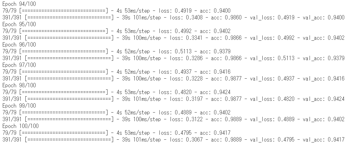
畳み込み層を行い残差ブロック54個とプーリング層を重ねます。(特徴の抽出)
次に、全結合を1つ重ねます。(分類)

1
2
3
4
5
6
7
8
9
10
11
12
13
14
15
16
17
18
19
20
21
22
23
# 入力データのシェイプ
input = Input(shape=(32,32, 3))

# 畳み込み層
x = conv(16, 3)(input)

# 残差ブロック x 54
x = residual_block(64, 1, 18)(x)
x = residual_block(128, 2, 18)(x)
x = residual_block(256, 2, 18)(x)

# →BN→ReLU
x = BatchNormalization()(x)
x = Activation('relu')(x)

# プーリング層
x = GlobalAveragePooling2D()(x)

# 全結合層
output = Dense(10, activation='softmax', kernel_regularizer=l2(0.0001))(x)

# モデルの作成
model = Model(inputs=input, outputs=output)

TPUモデルへの変換への変換を行います。

1
2
3
4
5
6
7
8
9
# TPUモデルへの変換
import tensorflow as tf
import os
tpu_model = tf.contrib.tpu.keras_to_tpu_model(
model,
strategy=tf.contrib.tpu.TPUDistributionStrategy(
tf.contrib.cluster_resolver.TPUClusterResolver(tpu='grpc://' + os.environ['COLAB_TPU_ADDR'])
)
)

コンパイルを行います。
損失関数はcategorical_crossentropy、最適化関数はSGD、評価指標accを設定します。

1
2
# コンパイル
tpu_model.compile(loss='categorical_crossentropy', optimizer=SGD(momentum=0.9), metrics=['acc'])

ImageDataGeneratorを使って、データセット画像の正規化と水増しを行います。

1
2
3
4
5
6
7
8
9
10
11
12
13
14
# ImageDataGeneratorの準備
train_gen = ImageDataGenerator(
featurewise_center=True,
featurewise_std_normalization=True,
width_shift_range=0.125,
height_shift_range=0.125,
horizontal_flip=True)
test_gen = ImageDataGenerator(
featurewise_center=True,
featurewise_std_normalization=True)

# データセット全体の統計量を予め計算
for data in (train_gen, test_gen):
data.fit(train_images)

LearningRateSchedulerを準備します。
LearningRateSchedulerは学習中に学習率を変化させるコールバックです。
学習率をはじめに0.1、80エポック以降0.01、120エポック以降0.001となるように設定します。
学習率は正解から遠い時には大きく、正解に近くなった時には小さく更新することで、速く正確に正解にだとりつけるように調整します。

1
2
3
4
5
6
7
# LearningRateSchedulerの準備
def step_decay(epoch):
x = 0.1
if epoch >= 80: x = 0.01
if epoch >= 120: x = 0.001
return x
lr_decay = LearningRateScheduler(step_decay)

訓練画像と訓練ラベルの配列をモデルに渡して、学習を行います。

1
2
3
4
5
6
7
8
9
# 学習
batch_size = 128
history = tpu_model.fit_generator(
train_gen.flow(train_images, train_labels, batch_size=batch_size),
epochs=100,
steps_per_epoch=train_images.shape[0] // batch_size,
validation_data=test_gen.flow(test_images, test_labels, batch_size=batch_size),
validation_steps=test_images.shape[0] // batch_size,
callbacks=[lr_decay])

実行結果6(途中略)

学習結果をグラフ表示します。

1
2
3
4
5
6
7
# グラフの表示
plt.plot(history.history['acc'], label='acc')
plt.plot(history.history['val_acc'], label='val_acc')
plt.ylabel('accuracy')
plt.xlabel('epoch')
plt.legend(loc='best')
plt.show()

実行結果7

テスト画像とテストラベルの配列をモデルに渡して評価を実行し、正解率を取得します。

1
2
3
4
5
6
# 評価
batch_size = 128
test_loss, test_acc = tpu_model.evaluate_generator(
test_gen.flow(test_images, test_labels, batch_size=batch_size),
steps=10)
print('loss: {:.3f}\nacc: {:.3f}'.format(test_loss, test_acc ))

実行結果8
正解率は94.2%となりました。
畳み込みニューラルネットワークでは73.5%だったのでかなりの性能向上です。


先頭10件のテスト画像の判定を行い、予測結果を表示します。
1
2
3
4
5
6
7
8
9
10
11
12
13
14
# 推論する画像の表示
for i in range(10):
plt.subplot(2, 5, i+1)
plt.imshow(test_images[i])
plt.show()

# 推論したラベルの表示
test_predictions = tpu_model.predict_generator(
test_gen.flow(test_images[0:16], shuffle = False, batch_size=16),
steps=16) # 学習データ数を16個に増やす
test_predictions = np.argmax(test_predictions, axis=1)[0:10] # 結果数を10個に減らす
labels = ['airplane', 'automobile', 'bird', 'cat', 'deer',
'dog', 'frog', 'horse', 'ship', 'truck']
print([labels[n] for n in test_predictions])

実行結果9

全ての画像を正しく判定できていることが分かります。

(Google Colaboratoryで動作確認しています。)

参考

AlphaZero 深層学習・強化学習・探索 人工知能プログラミング実践入門 サポートページ