深層学習でCIFAR10分類(一般物体認識)

CIFAR10とういうデータを使って一般物の認識をしてみます。

まずは必要なモジュールをインポートします。

1
2
3
4
5
6
7
8
9
10
import numpy as np
import matplotlib.pyplot as plt

import chainer.optimizers as Opt
import chainer.functions as F
import chainer.links as L
import chainer
import chainer.datasets as ds
import chainer.dataset.convert as con
from chainer import Variable, Chain, config, cuda

共通関数を定義します。

1
2
3
4
5
6
7
8
9
10
11
12
13
14
15
16
17
18
19
20
21
22
23
24
25
26
27
28
29
30
31
32
33
34
35
36
37
38
39
40
41
42
43
44
45
46
47
48
49
50
# -------------- #
# 共通関数の定義 #
# -------------- #
# データ振り分け関数
def data_divide(Dtrain, D, xdata, tdata, shuffle='on'):
if shuffle == 'on':
index = np.random.permutation(range(D))
elif shuffle == 'off':
index = np.arange(D)
else:
print('error')
xtrain = xdata[index[0:Dtrain],:]
ttrain = tdata[index[0:Dtrain]]
xtest = xdata[index[Dtrain:D],:]
ttest = tdata[index[Dtrain:D]]
return xtrain, xtest, ttrain, ttest

# グラフ表示関数
def show_graph(result1, result2, title, xlabel, ylabel, ymin=0.0, ymax=1.0):
# 学習記録の表示(誤差)
Tall = len(result1)
plt.figure(figsize=(12, 8))
plt.plot(range(Tall), result1, label='train')
plt.plot(range(Tall), result2, label='test')
plt.title(title)
plt.xlabel(xlabel)
plt.ylabel(ylabel)
plt.xlim([0, Tall])
plt.ylim(ymin, ymax)
plt.legend()
plt.show()

# 学習用関数
def learning_classification(model,optNN,data,result,T=10):
for time in range(T):
optNN.target.cleargrads()
ytrain = model(data[0])
loss_train = F.softmax_cross_entropy(ytrain,data[2])
acc_train = F.accuracy(ytrain,data[2])
loss_train.backward()
optNN.update()

with chainer.using_config('train', False), chainer.using_config('enable_backprop', False):
ytest = model(data[1])
loss_test = F.softmax_cross_entropy(ytest,data[3])
acc_test = F.accuracy(ytest,data[3])
result[0].append(cuda.to_cpu(loss_train.data))
result[1].append(cuda.to_cpu(loss_test.data))
result[2].append(cuda.to_cpu(acc_train.data))
result[3].append(cuda.to_cpu(acc_test.data))

一般物体認識のデータセットを読み込みます。

1
2
3
4
5
6
7
# 一般物体認識のデータセットの読み込み
train, test = ds.get_cifar10(ndim=3)
xtrain, ttrain = con.concat_examples(train)
xtest, ttest = con.concat_examples(test)

# データサイズの確認
Dtrain, ch, Ny, Nx = xtrain.shape

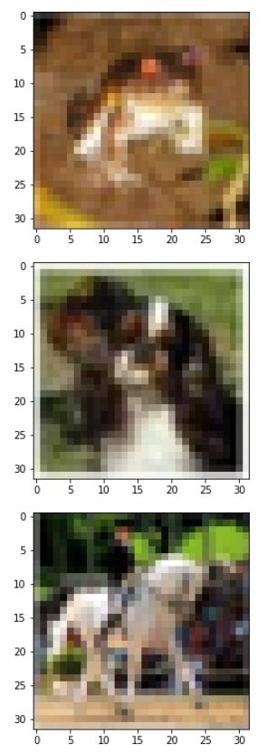
どんなデータがあるかいくつか画像を出力します。

1
2
3
4
5
6
7
8
9
# 試しに画像を出力
plt.imshow(xtrain[0,:,:,:].transpose(1, 2, 0))
plt.show()

plt.imshow(xtrain[500,:,:,:].transpose(1, 2, 0))
plt.show()

plt.imshow(xtrain[1200,:,:,:].transpose(1, 2, 0))
plt.show()

結果

画像識別の問題に有効な畳み込みニューラルネットワークを設定します。

1
2
3
4
5
6
7
8
9
# 2層畳み込みニューラルネットワークの設定
C = ttrain.max() + 1
H1 = 10

layers = {}
layers['conv1'] = L.Convolution2D(ch, H1, ksize=3, stride=1, pad=1)
layers['bnorm1'] = L.BatchRenormalization(H1)
layers['l1'] = L.Linear(None, C)
NN = Chain(**layers)

プーリング層を導入した関数を定義します。

1
2
3
4
5
6
7
8
# プーリング層の導入
def model(x):
h = NN.conv1(x)
h = F.relu(h)
h = NN.bnorm1(h)
h = F.max_pooling_2d(h, ksize=3, stride=2, pad=1)
y = NN.l1(h)
return y

GPUを設定します。

1
2
3
4
# GPUの設定
gpu_device = 0
cuda.get_device(gpu_device).use()
NN.to_gpu(gpu_device)

最適化手法を設定します。

1
2
3
# 最適化手法の設定
optNN = Opt.MomentumSGD()
optNN.setup(NN)

学習の経過を保存する変数を宣言します。

1
2
3
4
5
6
7
# 学習データ保存エリア
train_loss = []
train_acc = []
test_loss = []
test_acc = []

result = [train_loss, test_loss, train_acc, test_acc]

一度に全部実行するとメモリオーバーになってしまうのでデータセットを分割して実行します。
CIFARのデータは50,000個の訓練データがあるので5,000個ずつを10回に分けて実行します。

1
2
3
4
5
6
# シリアルイテレータの呼び出し
from chainer.iterators import SerialIterator as siter

# データセット振り分ける
batch_size = 5000
train_iter = siter(train, batch_size)

いつくかのバッチと呼ばれる小さな塊に分けて学習を進める方法をバッチ学習といいます。
特にランダムにデータを選んでニューラルネットワークの最適化を進める方法を確率勾配法といいます。
確率勾配法による最適化を行います。

1
2
3
4
5
6
7
# 確率勾配法による最適化
nepoch = 10
while train_iter.epoch < nepoch:
batch = train_iter.next()
xtrain, ttrain = con.concat_examples(batch)
data = cuda.to_gpu([xtrain, xtest, ttrain, ttest])
learning_classification(model, optNN, data, result, 1)

結果を表示します。

1
2
3
show_graph(result[0], result[1], 'loss function', 'step', 'loss function', 0.0, 4.0)

show_graph(result[2], result[3], 'accuracy', 'step', 'accuracy')

誤差

正解率

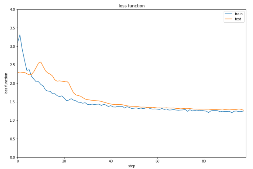
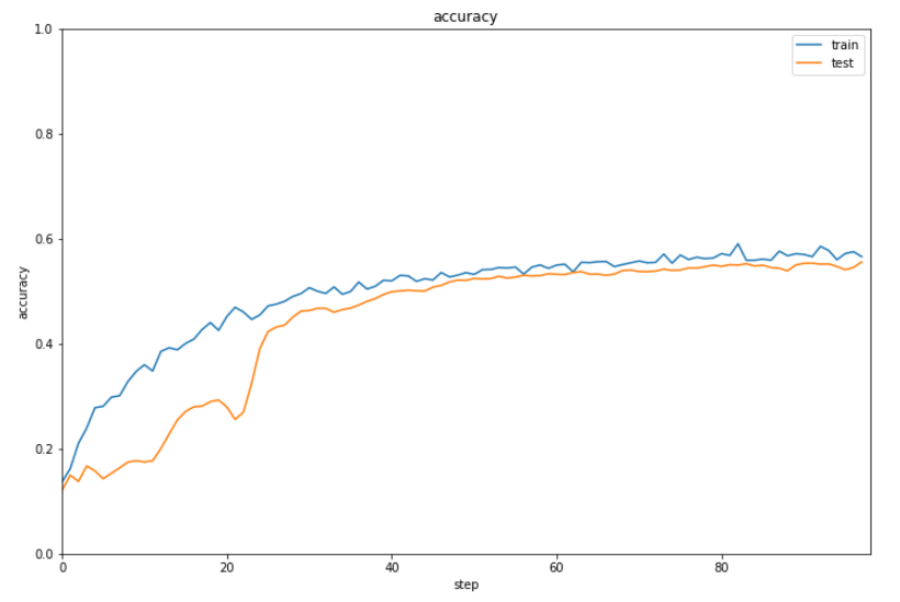
正解率は6割に届かない程度となりました。
ここから正解率を上げるために4層のニューラルネットワークにしていきます。

畳み込みニューラルネットワークのクラスを定義します。

1
2
3
4
5
6
7
8
9
10
11
12
13
14
# 畳み込みニューラルネットワークのクラス作成
class CNN(Chain):
def __init__(self, ch_in,ch_out):
layers = {}
layers['conv1'] = L.Convolution2D(ch_in,ch_out,ksize=5,stride=2,pad=2)
layers['bnorm1'] = L.BatchNormalization(ch_out)
super().__init__(**layers)

def __call__(self,x):
h = self.conv1(x)
h = self.bnorm1(h)
h = F.relu(h)

return h

多段階の畳み込みニューラルネットワークと関数を定義します。

1
2
3
4
5
6
7
8
9
10
11
12
13
14
15
16
17
18
19
20
21
22
23
24
25
26
27
28
29
30
31
32
33
34
35
36
37
38
39
40
41
42
43
44
45
46
47
48
49
50
51
52
53
54
55
# 多段階の畳み込みニューラルネットワーク
C = ttrain.max() + 1
H1 = 16
H2 = 32
H3 = 64

NN = Chain(cnn1 = L.Convolution2D(ch,H1,ksize=1,stride=1,pad=0),
cnn2 = L.Convolution2D(H1,H1,ksize=3,stride=1,pad=0),
cnn3 = L.Convolution2D(H1,H1,ksize=5,stride=1,pad=0),
cnn4 = L.Convolution2D(H1,H2,ksize=1,stride=1,pad=0),
cnn5 = L.Convolution2D(H2,H2,ksize=3,stride=1,pad=0),
cnn6 = L.Convolution2D(H2,H2,ksize=5,stride=1,pad=0),
cnn7 = L.Convolution2D(H2,H3,ksize=1,stride=1,pad=0),
cnn8 = L.Convolution2D(H3,H3,ksize=3,stride=1,pad=0),
cnn9 = L.Convolution2D(H3,C,ksize=5,stride=1,pad=3),
bnorm1 = L.BatchNormalization(H1),
bnorm2 = L.BatchNormalization(H1),
bnorm3 = L.BatchNormalization(H1),
bnorm4 = L.BatchNormalization(H2),
bnorm5 = L.BatchNormalization(H2),
bnorm6 = L.BatchNormalization(H2),
bnorm7 = L.BatchNormalization(H3),
bnorm8 = L.BatchNormalization(H3))

def model(x):
h = NN.cnn1(x)
h = F.relu(h)
h = NN.bnorm1(h)
h = NN.cnn2(h)
h = F.relu(h)
h = NN.bnorm2(h)
h = NN.cnn3(h)
h = F.relu(h)
h = NN.bnorm3(h)
h = F.max_pooling_2d(h, 2)
h = NN.cnn4(h)
h = F.relu(h)
h = NN.bnorm4(h)
h = NN.cnn5(h)
h = F.relu(h)
h = NN.bnorm5(h)
h = NN.cnn6(h)
h = F.relu(h)
h = NN.bnorm6(h)
h = F.max_pooling_2d(h, 2)
h = NN.cnn7(h)
h = F.relu(h)
h = NN.bnorm7(h)
h = NN.cnn8(h)
h = F.relu(h)
h = NN.bnorm8(h)
h = NN.cnn9(h)
y = F.mean(h,axis=(2,3))

return y

GPUの設定を行います。

1
2
3
4
# GPUの設定
gpu_device = 0
cuda.get_device(gpu_device).use()
NN.to_gpu()

結果を一旦初期化します。

1
2
3
4
5
train_loss = []
train_acc = []
test_loss = []
test_acc = []
result = [train_loss,train_acc,test_loss,test_acc]

最適化手法にAdamを設定します。

1
2
3
# 最適化手法の設定
optNN = Opt.Adam()
optNN.setup(NN)

関数を定義します。

1
2
3
4
5
6
7
8
9
10
11
12
13
14
15
16
17
18
19
20
21
22
23
24
25
26
27
28
29
def shift_labeled(labeled_data):
data, label = labeled_data

ch, Ny, Nx = data.shape
z_h = Ny * (2.0 * np.random.rand(1) - 1.0) * 0.3
z_v = Nx * (2.0 * np.random.rand(1) - 1.0) * 0.3
data = np.roll(data, int(z_h), axis=1)
data = np.roll(data, int(z_v), axis=2)

return data, label

def flip_labeled(labeled_data):
data, label = labeled_data
z = np.random.randint(2)
if z == 1:
data = data[:,::-1,:]
z = np.random.randint(2)
if z == 1:
data = data[:,:,::-1]

z = np.random.randint(2)
if z == 1:
data = data.transpose(0, 2, 1)
return data, label

def check_network(x, link):
print('input:', x.shape)
h = link(x)
print('output:', h.shape)

確率勾配法で最適化し、結果をグラフ化します。

1
2
3
4
5
6
7
8
9
10
11
12
13
14
15
16
17
from tqdm import tqdm

nepoch = 100
batch_size = 128
train_iter = siter(train, batch_size)
with tqdm(total = nepoch) as pbar:
while train_iter.epoch < nepoch:
pbar.update(train_iter.is_new_epoch)
batch = train_iter.next()
batch = ds.TransformDataset(batch, flip_labeled)
xtrain,ttrain = con.concat_examples(batch)
data = cuda.to_gpu([xtrain,xtest,ttrain,ttest])
learning_classification(model,optNN,data,result,1)
if train_iter.is_new_epoch == 1:
show_graph(result[0],result[1],'loss function in training','step','loss function',0.0,4.0)
show_graph(result[2],result[3],'Accuracy in training and test','step','accuracy')
print(result[3][len(result[3])-1])

2、3時間実行しているのですが、進捗が48%でまだ時間がかかるので一旦ここまでの結果を確認しておきます。
誤差
正解率

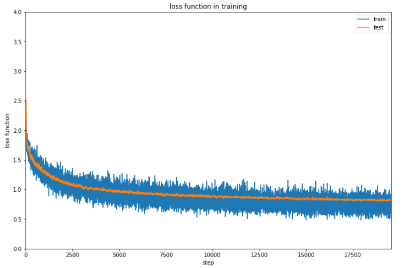
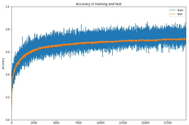
なんとか6割の正解率を超えてきているでしょうか。ただここまで時間がかかるのと正解率が微妙にしか上昇していないのでなんらかの改善の余地はあると思います。

5時間20分かかってようやく終了しました。
誤差
正解率

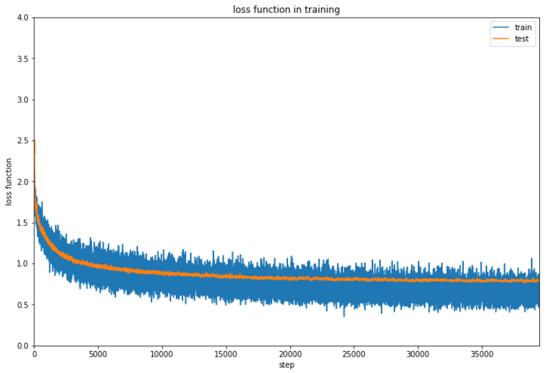
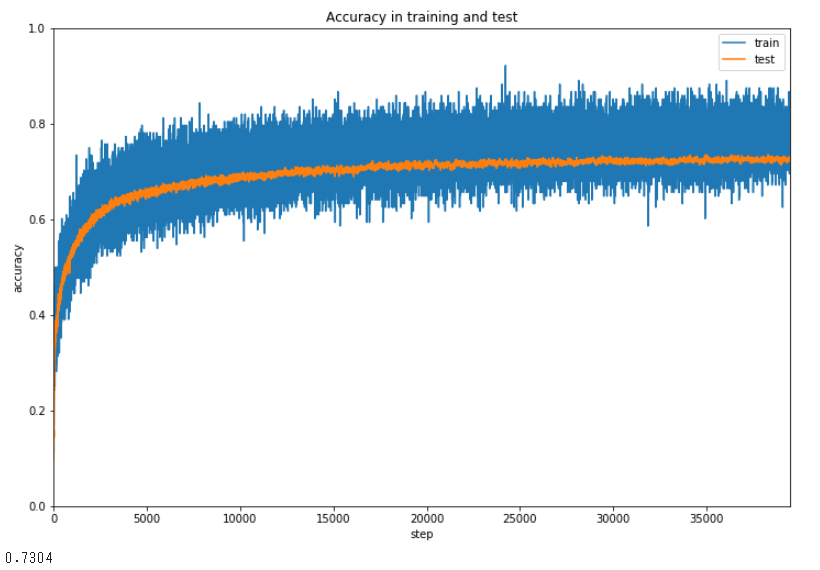
最終的な正解率は73%ですか。。。まー実用性があるといってもいいような気がします。

(Google Colaboratoryで動作確認しています。)