ニューラルネットワークで回帰分析をします。
1 2 3 4 5 6 7 8 9 10 11 12 13 14 15 16 17 18 19 20 21 22 23 24 25 26 27 28 29 30 31 32 33 34 35 36 37 38 39 40 41 42 43 44 45 46 47 48 49 50 51 52 53 54 55 import numpy as npimport matplotlib.pyplot as pltimport chainer.optimizers as Optimport chainer.functions as Fimport chainer.links as Lfrom chainer import Variable, Chain, config, cudadef data_divide (Dtrain, D, xdata, tdata ): index = np.random.permutation(range (D)) xtrain = xdata[index[0 :Dtrain],:] ttrain = tdata[index[0 :Dtrain]] xtest = xdata[index[Dtrain:D],:] ttest = tdata[index[Dtrain:D]] return xtrain, xtest, ttrain, ttest def show_graph (result1, result2, title, xlabel, ylabel, ymin=0.0 , ymax=1.0 ): Tall = len (result1) plt.figure(figsize=(8 , 6 )) plt.plot(range (Tall), result1, label='train' ) plt.plot(range (Tall), result2, label='test' ) plt.title(title) plt.xlabel(xlabel) plt.ylabel(ylabel) plt.xlim([0 , Tall]) plt.ylim(ymin, ymax) plt.legend() plt.show() def learning_regression (model, optNN, data, T=10 ): train_loss = [] test_loss = [] for time in range (T): config.train = True optNN.target.cleargrads() ytrain = model(data[0 ]) loss_train = F.mean_squared_error(ytrain, data[2 ]) loss_train.backward() optNN.update() config.train = False ytest = model(data[1 ]) loss_test = F.mean_squared_error(ytest, data[3 ]) train_loss.append(loss_train.data) test_loss.append(loss_test.data) return train_loss, test_loss
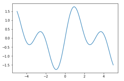
データを準備します。
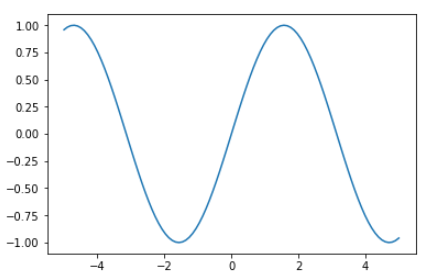
1 2 3 4 5 6 7 8 D = 100 ndata = np.linspace(-5.0 , 5.0 , D) N = 1 xdata = ndata.reshape(D, N).astype(np.float32) tdata = (np.sin(ndata) + np.sin(2.0 * ndata)).reshape(D, N).astype(np.float32)
作成したデータを視覚化します。
1 2 3 plt.plot(xdata, tdata) plt.show()
ニューラルネットワークを作成し関数化します。
1 2 3 4 5 6 7 8 9 10 11 C = 1 H = 20 NN = Chain(l1=L.Linear(N, H), l2=L.Linear(H, C), bnorm1=L.BatchNormalization(H)) def model (x ): h = NN.l1(x) h = F.relu(h) h = NN.bnorm1(h) y = NN.l2(h) return y
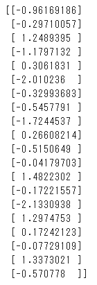
参考までに学習前のニューラルネットワークの状態を確認します。
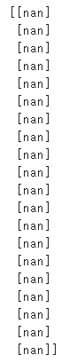
次に勾配を表示してみます。
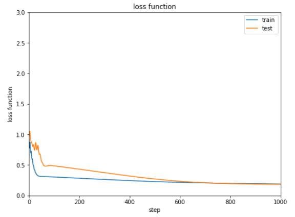
最適化手法を設定し学習を行います。
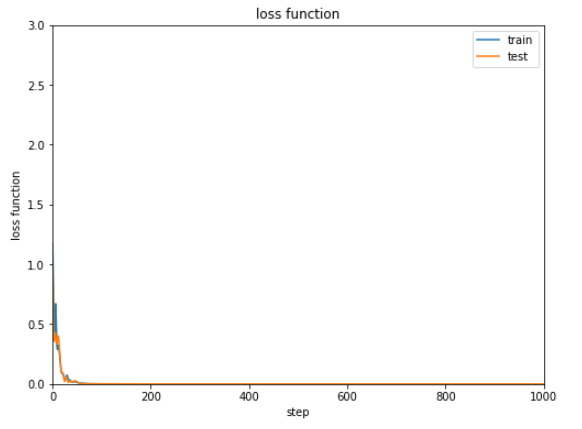
1 2 3 4 5 6 7 8 9 10 11 12 13 14 15 16 optNN = Opt.MomentumSGD() optNN.setup(NN) train_loss = [] test_loss = [] Dtrain = D // 2 xtrain, xtest, ttrain, ttest = data_divide(Dtrain, D, xdata, tdata) data = [xtrain, xtest, ttrain, ttest] result = [train_loss, test_loss] train_loss, test_loss = learning_regression(model, optNN, data, 1000 ) show_graph(train_loss, test_loss, 'loss function' , 'step' , 'loss function' , 0.0 , 3.0 )
学習結果の誤差は下記のようになります。
次第に減少してはいますが0.2から0.3付近で改善しなくなっています。
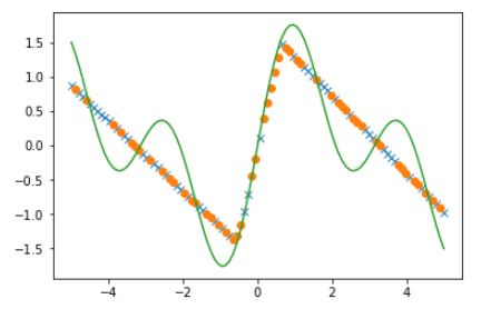
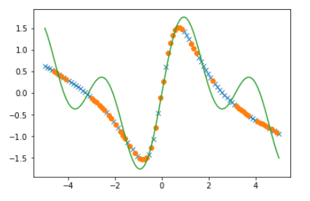
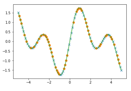
回帰の結果を比較します。
1 2 3 4 5 6 7 8 config.train = False ytrain = model(xtrain).data ytest = model(xtest).data plt.plot(xtrain, ytrain, marker='x' , linestyle='None' ) plt.plot(xtest, ytest, marker='o' , linestyle='None' ) plt.plot(xdata, tdata) plt.show()
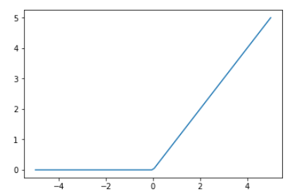
非線形関数調整してみます。
1 2 3 4 ydata = F.relu(xdata).data plt.plot(xdata, ydata) plt.show()
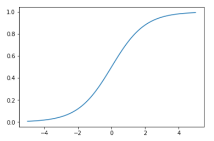
別の非線形関数sigmoidの形を調べると、reluよりは今回学習するデータに近いようにみえます。
1 2 3 4 ydata = F.sigmoid(xdata).data plt.plot(xdata, ydata) plt.show()
非線形関数をreluからsigmoidに変更し、同じように学習・結果表示を行います。
1 2 3 4 5 6 7 8 9 10 11 12 13 14 15 16 17 18 19 20 21 22 23 24 25 26 27 28 C = 1 H = 20 NN = Chain(l1=L.Linear(N, H), l2=L.Linear(H, C), bnorm1=L.BatchNormalization(H)) def model (x ): h = NN.l1(x) h = F.sigmoid(h) h = NN.bnorm1(h) h = NN.l2(h) return h optNN = Opt.MomentumSGD() optNN.setup(NN) train_loss = [] test_loss = [] Dtrain = D // 2 xtrain, xtest, ttrain, ttest = data_divide(Dtrain, D, xdata, tdata) data = [xtrain, xtest, ttrain, ttest] result = [train_loss, test_loss] train_loss, test_loss = learning_regression(model, optNN, data, 1000 ) show_graph(train_loss, test_loss, 'loss function' , 'step' , 'loss function' , 0.0 , 3.0 )
回帰の結果を確認してみます。
1 2 3 4 5 6 7 8 config.train = False ytrain = model(xtrain).data ytest = model(xtest).data plt.plot(xtrain, ytrain, marker='x' , linestyle='None' ) plt.plot(xtest, ytest, marker='o' , linestyle='None' ) plt.plot(xdata, tdata) plt.show()
ただまだまだ納得いく結果ではありません。
1 2 3 4 ydata = F.sin(xdata).data plt.plot(xdata, ydata) plt.show()
非線形関数をsinに変更してまたまた回帰分析を行います。
1 2 3 4 5 6 7 8 9 10 11 12 13 14 15 16 17 18 19 20 21 22 23 24 25 26 27 28 C = 1 H = 20 NN = Chain(l1=L.Linear(N, H), l2=L.Linear(H, C), bnorm1=L.BatchNormalization(H)) def model (x ): h = NN.l1(x) h = F.sin(h) h = NN.bnorm1(h) h = NN.l2(h) return h optNN = Opt.MomentumSGD() optNN.setup(NN) train_loss = [] test_loss = [] Dtrain = D // 2 xtrain, xtest, ttrain, ttest = data_divide(Dtrain, D, xdata, tdata) data = [xtrain, xtest, ttrain, ttest] result = [train_loss, test_loss] train_loss, test_loss = learning_regression(model, optNN, data, 1000 ) show_graph(train_loss, test_loss, 'loss function' , 'step' , 'loss function' , 0.0 , 3.0 )
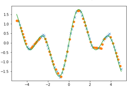
回帰の結果も確認してみます。
1 2 3 4 5 6 7 8 config.train = False ytrain = model(xtrain).data ytest = model(xtest).data plt.plot(xtrain, ytrain, marker='x' , linestyle='None' ) plt.plot(xtest, ytest, marker='o' , linestyle='None' ) plt.plot(xdata, tdata) plt.show()
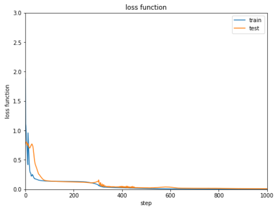
relu関数のまま結果を改善することはできないのでしょうか。
1 2 3 4 5 6 7 8 9 10 11 12 13 14 15 16 17 18 19 20 21 22 23 24 25 26 27 28 29 30 31 32 33 34 35 36 37 38 39 40 41 42 43 44 45 46 47 48 49 50 51 52 53 C = 1 H1 = 5 H2 = 5 H3 = 5 layers = {} layers['l1' ] = L.Linear(N, H1) layers['l2' ] = L.Linear(H1, H2) layers['l3' ] = L.Linear(H2, H3) layers['l4' ] = L.Linear(H3, C) layers['bnorm1' ] = L.BatchNormalization(H1) layers['bnorm2' ] = L.BatchNormalization(H2) layers['bnorm3' ] = L.BatchNormalization(H3) NN = Chain(**layers) def model (x ): h = NN.l1(x) h = F.relu(h) h = NN.bnorm1(h) h = NN.l2(h) h = F.relu(h) h = NN.bnorm2(h) h = NN.l3(h) h = F.relu(h) h = NN.bnorm3(h) y = NN.l4(h) return y optNN = Opt.MomentumSGD() optNN.setup(NN) train_loss = [] test_loss = [] Dtrain = D // 2 xtrain, xtest, ttrain, ttest = data_divide(Dtrain, D, xdata, tdata) data = [xtrain, xtest, ttrain, ttest] result = [train_loss, test_loss] train_loss, test_loss = learning_regression(model, optNN, data, 1000 ) show_graph(train_loss, test_loss, 'loss function' , 'step' , 'loss function' , 0.0 , 3.0 ) config.train = False ytrain = model(xtrain).data ytest = model(xtest).data plt.plot(xtrain, ytrain, marker='x' , linestyle='None' ) plt.plot(xtest, ytest, marker='o' , linestyle='None' ) plt.plot(xdata, tdata) plt.show()
結果は以下の通りです。
(Google Colaboratory で動作確認しています。)