Balancing Security, Operating Cost, and Performance
Rotate keys too rarely and a single leaked key exposes years of data. Rotate too often and you drown in operational overhead, re-encryption jobs, and latency spikes. Somewhere between those extremes lies an interval that minimizes total cost. In this post we build a cost model for key rotation, derive the optimal interval analytically, verify it numerically, and stress-test it with a Monte Carlo simulation of random key-compromise events.
The Problem Setup
Imagine a platform that manages $N = 50$ data-encryption keys, each protecting a different data store. We must choose a single rotation interval $T$ (in days). Three cost components matter.
1. Operational cost. Every rotation cycle has a fixed overhead $C_f$ (change approval, audit logging, KMS orchestration) plus a per-key cost $C_o$ (re-wrapping, distribution, verification). The number of cycles per year is $365/T$:
$$
C_{\text{ops}}(T) = \frac{365}{T}\left(C_f + N,C_o\right)
$$
2. Performance cost. Each rotation triggers re-encryption or cache invalidation, causing latency spikes and extra compute. We model this as a per-key cost $C_p$ per rotation:
$$
C_{\text{perf}}(T) = \frac{365}{T},N,C_p
$$
3. Security risk cost. Suppose key compromise events occur at a rate of $\lambda$ per year. A leaked key can be abused until it is rotated, so the exposure window grows with $T$. If each day of exposure costs $V$ dollars in expected damage, the expected annual loss is proportional to $T$:
$$
C_{\text{risk}}(T) = \lambda,V,T
$$
The total annual cost is therefore
$$
C(T) = \frac{365\left(C_f + N,(C_o + C_p)\right)}{T} + \lambda,V,T
$$
Closed-Form Optimum
Let $A = 365\left(C_f + N(C_o + C_p)\right)$ and $B = \lambda V$. Then $C(T) = A/T + BT$. Setting the derivative to zero:
$$
\frac{dC}{dT} = -\frac{A}{T^2} + B = 0 \quad\Longrightarrow\quad T^{*} = \sqrt{\frac{A}{B}} = \sqrt{\frac{365\left(C_f + N(C_o + C_p)\right)}{\lambda,V}}
$$
The minimum cost is
$$
C(T^{*}) = 2\sqrt{AB}
$$
Because $C’’(T) = 2A/T^3 > 0$, this stationary point is a global minimum. The structure is the same as the classic economic order quantity (EOQ) model: fixed cost per cycle versus holding cost that grows with cycle length.
Parameters Used
| Symbol | Meaning | Value |
|---|---|---|
| $N$ | Number of managed keys | 50 |
| $C_f$ | Fixed cost per rotation cycle | $800 |
| $C_o$ | Operational cost per key per rotation | $120 |
| $C_p$ | Performance cost per key per rotation | $30 |
| $\lambda$ | Key-compromise rate (events/year) | 0.25 |
| $V$ | Expected damage per exposure-day | $4,000 |
Monte Carlo Extension
The analytic model uses expected values only. Real security teams also care about the tail. In the simulation, the number of compromise events per year follows a Poisson distribution with mean $\lambda$, and each event has a log-normal severity multiplier $S$ with $\mathbb{E}[S] = 1$:
$$
S \sim \text{LogNormal}!\left(-\tfrac{\sigma^2}{2},\ \sigma^2\right), \qquad \sigma = 0.8
$$
$$
L(T) = V,T\sum_{i=1}^{K} S_i, \qquad K \sim \text{Poisson}(\lambda)
$$
We then compare the interval that minimizes the expected cost with the one that minimizes the 95th-percentile cost.
The Complete Source Code
All the code lives in a single cell. The Monte Carlo part is fully vectorized (Poisson counts, log-normal severities, and np.bincount aggregation), so 100,000 simulated years across 40 candidate intervals finishes in seconds.
1 | import numpy as np |
Code Walkthrough
1. Parameters and cost functions
The constants at the top map one-to-one to the table above. The four small functions implement the equations directly:
op_costis $\frac{365}{T}(C_f + N C_o)$.perf_costis $\frac{365}{T} N C_p$.risk_costis $\lambda V T$.total_costadds the three together.
Each function takes T as either a scalar or a NumPy array, and n and lam as optional arguments. This matters later, because the 3D surfaces are built by passing whole meshgrids through the same functions.
t_star is the closed-form solution $T^* = \sqrt{A/B}$, also vectorized in $N$ and $\lambda$, so we can draw the optimal interval as a surface.
2. Optimization three ways
We find the optimum in three ways:
- Analytic:
t_star(). - Numerical:
minimize_scalarwith the bounded (Brent-type) method over $[1, 365]$ days, with a very tight tolerance. It should agree with the formula to many decimal places. - Integer-day brute force: evaluating every whole-day interval from 1 to 365 and taking
argmin. This is the answer you would actually deploy, since cron-style schedules usually work in whole days.
Agreement between all three is a cheap sanity check that the derivation and the code match.
3. Policy comparison
Real organizations rarely pick 55 days. They pick a policy name: daily, weekly, monthly, quarterly, and so on. The loop prints each policy’s cost components and its percentage penalty over the optimum, and stores the totals for the bar chart.
4. Vectorized Monte Carlo
For each candidate interval we simulate 100,000 years:
rng.poisson(LAMBDA, N_SIMS)draws the number of compromise events in each simulated year.rng.lognormal(...)draws one severity value per event. Setting the log-mean to $-\sigma^2/2$ makes $\mathbb{E}[S] = 1$, so the Monte Carlo mean is directly comparable to the analytic model.np.repeat(np.arange(N_SIMS), counts)labels each severity with the simulated year it belongs to, andnp.bincount(..., weights=sev)sums severities per year without a Python loop.- Multiplying by $V \cdot T$ converts severity into dollars.
This is the speed-up. A naive double loop over years and events would take minutes. The vectorized version handles 40 intervals × 100,000 years in a few seconds. The fixed (operations and performance) costs are deterministic, so only the loss term is random.
We record two statistics per interval: the mean total cost and the 95th-percentile total cost.
5. The six-panel dashboard
Everything is drawn in one figure so you only need to paste a single image:
- (a) Cost decomposition for the three components and the total.
- (b) A 3D surface of total cost over $T$ and $\lambda$, with the optimum curve traced on top.
- (c) A 3D surface of $T^*$ over fleet size $N$ and compromise rate $\lambda$.
- (d) Monte Carlo curves against the analytic expectation.
- (e) Cost curves for four fleet sizes, with optima marked.
- (f) A log-scale bar chart of common rotation policies.
Results
Console output
=== Optimal rotation interval ===
Analytic  T* =   55.041 days
Numerical T* =   55.041 days  (cost = $110,082/year)
Integer-day optimum = 55 days  (cost = $110,082/year)

=== Policy comparison ===
Policy        T[d]          Op        Perf        Risk       Total   vs opt
Daily            1   2,482,000     547,500       1,000   3,030,500  2653.0%
Weekly           7     354,571      78,214       7,000     439,786   299.5%
Monthly         30      82,733      18,250      30,000     130,983    19.0%
Quarterly       90      27,578       6,083      90,000     123,661    12.3%
Semi-annual    180      13,789       3,042     180,000     196,831    78.8%
Annual         365       6,800       1,500     365,000     373,300   239.1%

=== Monte Carlo ===
Best T (expected cost) : 60 days ($109,989)
Best T (95th pct cost) : 20 days ($272,690)
Figure
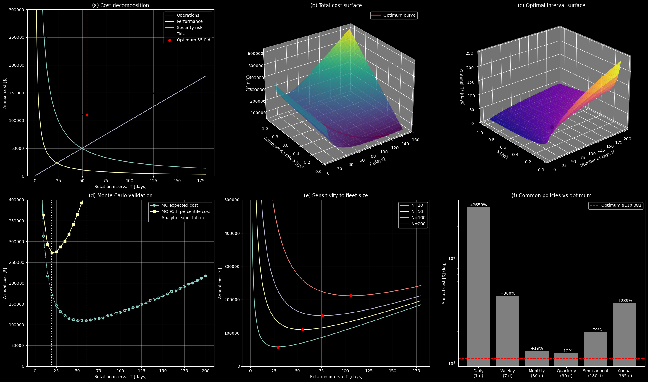
Interpreting the Results
The optimum is about 55 days
The closed-form, numerical, and brute-force answers all land at $T^* \approx 55$ days, with a minimum annual cost of roughly $110,082. Plugging in the numbers:
$$
A = 365 \times (800 + 50 \times 150) = 3{,}029{,}500, \qquad B = 0.25 \times 4000 = 1000
$$

At the optimum, the rotation-related costs ($A/T$) and the risk cost ($BT$) are exactly equal, about $55,041 each. That equality is a useful rule of thumb: at the optimum, the “cost of rotating” and the “cost of waiting” balance.
Panel (a): the U-shaped total cost
The operations and performance curves fall like $1/T$ and the risk line rises linearly. Their sum is a smooth U shape with a flat bottom. The flatness is important in practice: you do not need to hit 55.04 days exactly. Anything from roughly 40 to 75 days stays within about 10% of the minimum.
Panel (b): how the cost landscape moves with threat level
The 3D surface shows total cost over rotation interval $T$ and compromise rate $\lambda$. For a high $\lambda$ (a hostile threat environment), the valley shifts toward short intervals and the walls rise steeply on the long-interval side. For a low $\lambda$, the valley is wide and shallow. The red curve is the analytic optimum, and it sits precisely at the bottom of the valley for every $\lambda$.
Panel (c): the optimal interval surface
Because $T^* \propto \sqrt{N/\lambda}$ (for large $N$), the optimal interval grows with the square root of fleet size and shrinks with the square root of threat level. The black dot marks our scenario. Two consequences follow:
- Doubling your key count does not double the optimal interval, only multiplies it by about $\sqrt{2} \approx 1.41$.
- A 4× increase in compromise likelihood halves the optimal interval.
Panel (d): Monte Carlo validation and the tail
The Monte Carlo mean tracks the analytic curve closely, which validates the model. The best interval under expected cost comes out at 60 days (about $109,989 in this simulation), consistent with the 55-day analytic result given the 5-day grid and sampling noise.
The 95th-percentile curve tells a different story. Because compromise events are rare but severe, the tail cost is dominated by the loss term, and its minimum shifts to a much shorter interval of about 20 days (about $272,690). A risk-averse organization that budgets for the bad year, not the average year, should rotate far more often than the expected-cost model suggests. The two optima bracket the real decision: the 20-day tail-protective interval at the short end and the 55-to-60-day expected-cost interval at the long end.
Panel (e): sensitivity to fleet size
Larger fleets shift the optimum to the right and raise the whole cost curve. With 200 keys, per-cycle overhead is large, so you rotate less often. With 10 keys, rotation is cheap and the optimum moves left. This is why large organizations often adopt tiered rotation: frequent rotation for a small set of crown-jewel keys, and longer intervals for the long tail.
Panel (f): what common policies cost
| Policy | Interval | Total cost | vs optimum |
|---|---|---|---|
| Daily | 1 day | $3,030,500 | +2653% |
| Weekly | 7 days | $439,786 | +300% |
| Monthly | 30 days | $130,983 | +19% |
| Quarterly | 90 days | $123,661 | +12% |
| Semi-annual | 180 days | $196,831 | +79% |
| Annual | 365 days | $373,300 | +239% |
Rotating daily costs nearly 28 times the optimum, almost entirely from operations and performance overhead. Rotating annually costs more than 3 times the optimum, almost entirely from risk. Monthly and quarterly schedules, the ones most compliance frameworks nudge you toward, happen to sit close to the sweet spot for this particular parameter set, at +19% and +12%. The log-scale axis is needed here because the extremes differ from the optimum by orders of magnitude.
Practical Takeaways
- Rotation frequency is an economics problem, not just a compliance checkbox. The $\sqrt{A/B}$ structure gives you a defensible starting point you can explain to auditors and finance alike.
- The curve is flat near the optimum. Choose a round, operationally convenient number near $T^*$ rather than agonizing over the exact value.
- Reduce fixed costs and the optimum drops. Automating rotation (lowering $C_f$ and $C_o$) lets you rotate more often at the same budget. Investing in automation is, in effect, buying security.
- Decide your risk appetite explicitly. Expected-cost optimization and tail-risk optimization give different answers (about 55 days versus 20 days here). The gap between them is the price of insurance against the bad year.
- Re-estimate $\lambda$ and $V$ regularly. Because $T^* \propto 1/\sqrt{\lambda V}$, a change in threat intelligence or data sensitivity should move your rotation schedule, even if the change is modest.