Shrinking Permission Matrices Without Slowing Anyone Down
Every organization eventually suffers from privilege creep. People change teams, projects end, and temporary grants quietly become permanent. Years later, an engineer who only needs read access to a repository can also deploy to production, and an accounts-payable clerk can both create and approve the same invoice.
The principle of least privilege says everyone should hold exactly the permissions they need and nothing more. Applying it blindly causes the opposite problem: people get blocked, tickets pile up, and productivity drops. In this article we model the trade-off as a mixed-integer linear program (MILP) and solve a concrete example with Python.
1. The Problem Setting
We have an organization with $U = 40$ users in five departments (Sales, Engineering, Finance, HR, Support) and $P = 16$ permissions such as CRM_Read, Prod_Deploy, DB_Admin, and Payroll_Edit.
- Granted matrix $g_{up}\in{0,1}$: permission $p$ is currently granted to user $u$.
- Need matrix $n_{up}\in{0,1}$: user $u$ actually uses permission $p$ in their work.
- Usage frequency $f_{up}$: how many times per month user $u$ uses permission $p$.
- Critical flag $c_{up}=1$ if $f_{up}\ge 8$. These permissions are essential to the daily job and must never be revoked.
- Risk weight $r_p$ is the severity of permission $p$, and $e_u$ is the exposure of user $u$ (for example, 1.5 for contractors).
- Just-in-time (JIT) friction cost: if a needed but non-critical permission is revoked, the user must request temporary access each time, which costs $\tau$ per use.
The decision variable is the final matrix $x_{up}\in{0,1}$, where $x_{up}=1$ means “keep the permission”.
2. Mathematical Formulation
The residual security risk and the productivity loss are
$$
\mathrm{Risk}(x)=\sum_{u=1}^{U}\sum_{p=1}^{P} r_p,e_u,x_{up},
\qquad
\mathrm{Loss}(x)=\sum_{u=1}^{U}\sum_{p=1}^{P} n_{up},\tau f_{up},(1-x_{up}).
$$
We minimize a weighted sum of the two, where $\lambda$ controls how much we value productivity relative to security:
$$
\min_{x}\ \ \mathrm{Risk}(x)+\lambda,\mathrm{Loss}(x)
$$
subject to
$$
c_{up}\le x_{up}\le g_{up}\qquad\forall u,p \quad (\text{keep critical permissions, never add new ones})
$$
$$
x_{ua}+x_{ub}\le 1\qquad\forall u,\ \forall (a,b)\in\mathcal{S} \quad (\text{separation of duties})
$$
$$
\sum_{u=1}^{U}x_{up}\le K_p\qquad\forall p\in\mathcal{H} \quad (\text{holder cap on high-risk permissions})
$$
$$
x_{up}\in{0,1}.
$$
Here $\mathcal{S}$ is the set of conflicting permission pairs: (Inv_Create, Inv_Approve), (Src_Write, Prod_Deploy), and (User_Admin, Audit_Read). $\mathcal{H}$ is the set of high-risk permissions, and $K_p$ is the maximum number of holders allowed for permission $p$.
Substituting $n_{up}\tau f_{up}(1-x_{up}) = n_{up}\tau f_{up}-n_{up}\tau f_{up},x_{up}$ turns the objective into a linear function of $x$ plus a constant:
$$
\min_x \sum_{u,p}\Big(r_p e_u-\lambda,n_{up}\tau f_{up}\Big)x_{up}.
$$
Each coefficient has a clear meaning. A permission is worth keeping only when the friction it removes, $\lambda n_{up}\tau f_{up}$, outweighs the risk it adds, $r_p e_u$. The constraints then decide the cases where that simple rule is not allowed to win.
3. Why a MILP, and Why It Is Fast
A naive search over all subsets of granted permissions needs $2^n$ evaluations, where $n$ is the number of granted entries. With hundreds of entries that is hopeless. Three design choices keep the computation light:
- Variable pruning. Only entries with $g_{up}=1$ become variables. Entries that are not granted are fixed at zero and never enter the model.
- Fixed lower bounds. Critical entries get a lower bound of 1, so the solver never has to explore them.
- HiGHS through SciPy.
scipy.optimize.milpuses the HiGHS solver, which solves this problem in milliseconds. That makes it practical to repeat the solve 31 times to trace the entire Pareto frontier.
4. Complete Source Code
1 | import time |
5. Code Walkthrough
5.1 Data generation
Each department has a list of core permissions, which are used heavily (8 to 20 times a month) and are therefore critical. It also has a list of occasional permissions, which a user needs with 70% probability at low frequency (1 to 7 times a month). The random generator is seeded, so every run produces exactly the same organization.
Because separation-of-duties pairs are hard constraints, the code demotes one permission of any pair that a user holds as critical. This guarantees a feasible solution always exists: keeping only the critical permissions satisfies every constraint.
5.2 Modeling privilege creep
The granted matrix G starts from the need matrix N and adds extra grants with 30% probability per cell. These extras represent leftover permissions from old projects and one-time approvals. They carry risk but give no productivity benefit, which is the waste we want to eliminate.
5.3 Risk and friction matrices
R = np.outer(exposure, RISK) implements $r_p e_u$ for all users and permissions at once. L = usage * JIT_COST implements $\tau f_{up}$, and NL applies the need mask so that friction is only charged where a permission was actually used.
5.4 The MILP
Inside solve, np.argwhere(G == 1) lists the granted entries, and vid maps each (user, permission) pair to a variable index. The objective vector c is exactly the coefficient $r_pe_u-\lambda n_{up}\tau f_{up}$ derived earlier.
- Bounds
lb/ubencode $c_{up}\le x_{up}\le g_{up}$. - Separation of duties adds one row per user and conflicting pair, with right-hand side 1.
- Holder caps add one row per high-risk permission that sums that column of variables, with right-hand side $K_p$.
integrality=np.ones(n)makes every variable binary, since the bounds restrict it to $[0,1]$.
The cap $K_p$ is set to the larger of 4 and the number of critical holders, so it can never contradict the lower bounds.
5.5 Metrics
metrics evaluates any candidate matrix on the same scale: granted count, excess grants, residual risk, productivity loss, separation-of-duties violations, cap violations, and unmet critical needs. This lets us compare three scenarios fairly: the current state, a simple usage-based revoke heuristic (keep exactly what people use), and the MILP optimum.
5.6 The Pareto sweep
Sweeping $\lambda$ from $10^{-1.5}$ to $10^{1.5}$ in 31 steps traces the whole frontier. A small $\lambda$ treats friction as cheap, so almost everything non-critical is revoked. A large $\lambda$ treats friction as expensive, so every permission anyone actually uses is kept. The operating point $\lambda=1$ balances the two.
5.7 The figure
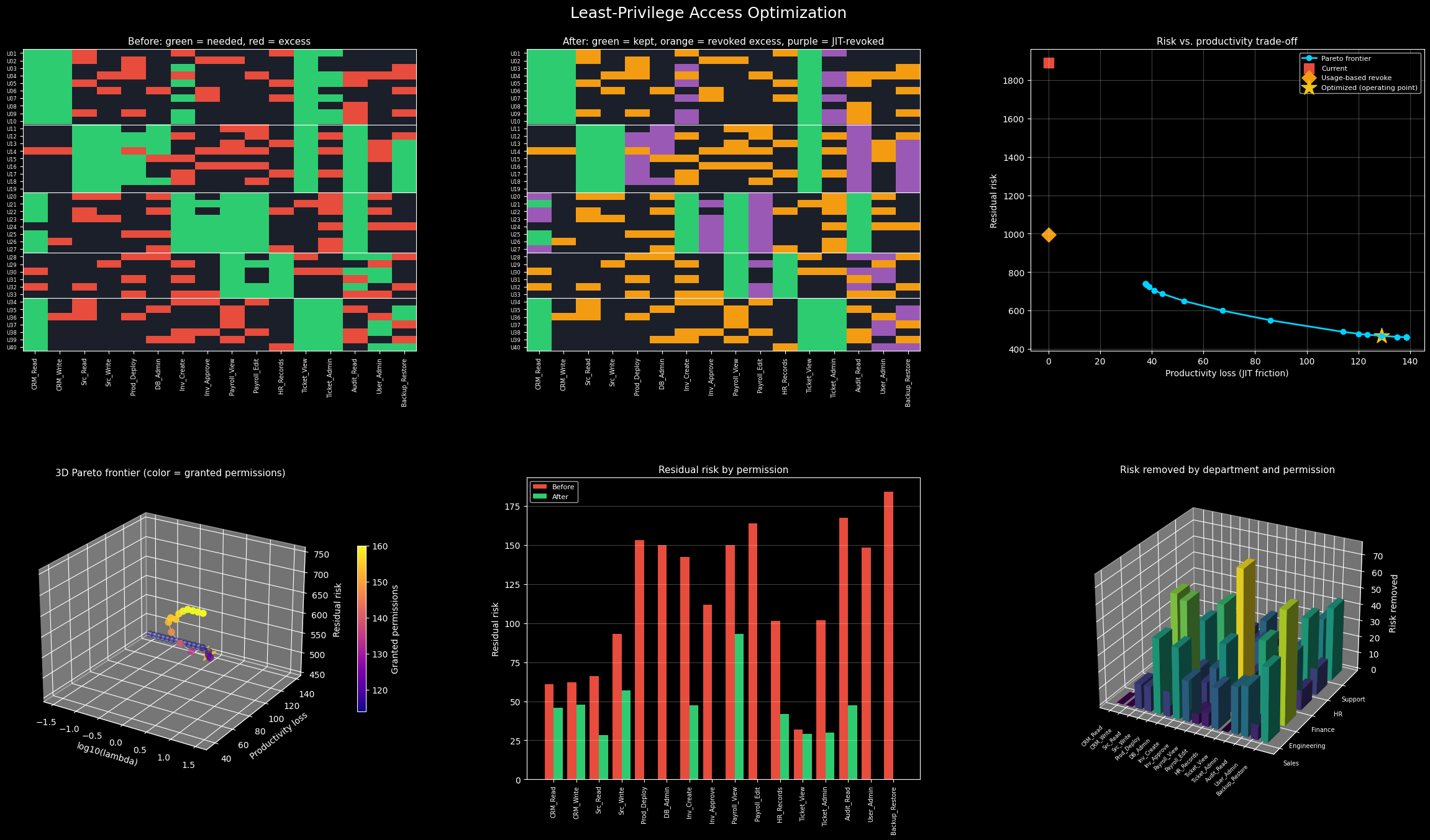
All six panels are drawn into a single figure. The two heatmaps use categorical color codes, so each cell tells you its status at a glance. The Pareto panel and the 3D panel come from the sweep, and the last two panels aggregate the effect of the optimization by permission and by department.
6. Execution Results
6.1 Result Image
6.2 Console Output
=== Dataset ===
Users: 40 | Permissions: 16 | Granted: 317 | Needed: 188 | Critical: 114 | Excess: 129
Pareto sweep: 31 MILP solves in 0.13 s

=== Scenario comparison (lambda = 1.0) ===
                       Granted  Excess  Residual risk  Productivity loss  SoD violations  Cap violations  Critical unmet
Current (all granted)    317.0   129.0         1889.0                0.0            30.0             5.0             0.0
Usage-based revoke       188.0     0.0          995.0                0.0            14.0             5.0             0.0
Optimized (MILP)         117.0     0.0          468.5              129.0             0.0             0.0             0.0

=== By department ===
 Department  Users  Granted before  Granted after  Risk before  Risk after
      Sales     10              72             30        390.5        84.0
Engineering      9              82             27        490.5        95.0
    Finance      8              69             27        463.5       159.0
         HR      6              42             12        266.0        78.0
    Support      7              52             21        278.5        52.5

=== Highest-risk revoked grants ===
U06 (Sales      ) DB_Admin       risk= 15.0  needed=N
U39 (Support    ) DB_Admin       risk= 15.0  needed=N
U03 (Sales      ) Prod_Deploy    risk= 13.5  needed=N
U09 (Sales      ) Prod_Deploy    risk= 13.5  needed=N
U24 (Finance    ) User_Admin     risk= 13.5  needed=N
U03 (Sales      ) Backup_Restore risk= 12.0  needed=N
U06 (Sales      ) Backup_Restore risk= 12.0  needed=N
U09 (Sales      ) Backup_Restore risk= 12.0  needed=N
–
7. How to Read the Results
7.1 Heatmaps: before and after
In the left heatmap, red cells are excess grants that nobody uses. They are scattered across every department, which is the visual signature of privilege creep. In the center heatmap, the red cells have turned into orange cells, meaning they were revoked at no productivity cost. Purple cells, if any appear, mark permissions that people did use occasionally but that were revoked because their risk outweighed the JIT friction, or because a separation-of-duties or holder-cap constraint forced the decision. Green cells are the permissions that survive.
7.2 The trade-off curve
The 2D Pareto plot shows that no single scenario wins on both axes:
- Current state has zero productivity loss and the highest risk.
- Usage-based revoke removes every unused grant but still ignores separation of duties and holder caps, so the console table shows nonzero constraint violations for it. Removing unused permissions is therefore necessary but not sufficient.
- The MILP optimum (the star) sits on the frontier and, unlike the heuristic, satisfies every constraint. It accepts a small amount of JIT friction in exchange for removing the riskiest remaining grants.
The frontier is steep at first and flattens afterwards: the first reductions in risk cost almost nothing, and only the last ones require real friction. This is why the operating point should sit near the bend rather than at either extreme.
7.3 The 3D Pareto frontier
The third axis shows $\log_{10}\lambda$ explicitly, and color shows the number of granted permissions. Moving along the curve is moving along the policy dial: low $\lambda$ gives a lean, strict matrix with more friction, and high $\lambda$ gives a permissive matrix with less friction. The star marks the chosen policy, and you can see how many grants it keeps relative to both ends.
7.4 Risk by permission
The bar chart shows which permissions carried the most risk before and after. High-weight permissions such as DB_Admin, Prod_Deploy, User_Admin, and Payroll_Edit show the largest reductions, because their risk coefficients are large enough to outweigh friction for rarely used grants. Low-risk permissions such as Ticket_View barely change.
7.5 Risk removed by department and permission
The 3D bar chart shows where the cleanup happens. Tall bars mark department–permission combinations where large amounts of risk were removed. This view is useful in practice because it turns an optimization result into a work list: the tallest bars are the access reviews that deserve attention first.
8. Practical Takeaways
- Treat least privilege as an optimization, not a slogan. Revoking everything unused is cheap to compute but ignores separation of duties and holder limits. Putting these in the model makes the result compliant by construction.
- Protect critical work with hard constraints. Lower bounds on daily-use permissions guarantee that the optimization can never cripple a job, no matter how $\lambda$ is set.
- Price friction honestly. JIT access is the pressure valve that makes aggressive revocation tolerable. The model quantifies exactly how much friction each risk reduction costs.
- Choose the policy from the frontier. Instead of arguing about a single threshold, the Pareto curve lets security and operations teams pick a point together and see what each side gives up.
- Scale is not a problem. Pruning to granted entries and using a modern MILP solver means the same formulation extends to thousands of users and hundreds of permissions, and the sweep can be rerun every time the access data is refreshed.
9. Conclusion
We turned the least-privilege principle into a binary linear program that minimizes residual risk plus weighted productivity loss, subject to critical-access, separation-of-duties, and holder-cap constraints. Solving it with HiGHS through SciPy takes milliseconds, which allowed us to sweep $\lambda$ and visualize the full risk–productivity frontier in 2D and 3D. The result is a defensible, quantitative answer to the question every access review asks: which permissions can we take away without anyone noticing?