Maximizing Quantum Fisher Information with Python
How precisely can you measure a phase with $N$ qubits? The answer depends on two design choices: which input state you prepare and which measurement you perform. In this post we work through a concrete example, an $N$-qubit phase estimator, and solve the probe design problem numerically, both without noise and under local dephasing.
1. The Problem
A parameter $\varphi$ is imprinted on a probe state through the unitary
$$
U_\varphi = e^{-i\varphi G}, \qquad G=\frac12\sum_{i=1}^{N}\sigma_z^{(i)} .
$$
The quantum Cramér–Rao bound limits the variance of any unbiased estimator after $\nu$ repetitions:
$$
\mathrm{Var}(\hat\varphi);\ge;\frac{1}{\nu,F_Q[\rho_\varphi]} .
$$
The quantum Fisher information (QFI) $F_Q$ depends only on the probe state. For a pure state it is
$$
F_Q = 4\left(\langle G^2\rangle-\langle G\rangle^2\right).
$$
For a mixed state $\rho=\sum_i\lambda_i|i\rangle\langle i|$ it becomes
$$
F_Q = 2\sum_{i,j}\frac{(\lambda_i-\lambda_j)^2}{\lambda_i+\lambda_j},\big|\langle i|G|j\rangle\big|^2 .
$$
Step 1: Choosing the input state
The eigenvalues of $G$ range from $-N/2$ to $+N/2$, so the variance is bounded by $\mathrm{Var}(G)\le N^2/4$ and therefore
$$
F_Q\le N^2 \quad(\text{Heisenberg limit}).
$$
A product state such as $|+\rangle^{\otimes N}$ only reaches $F_Q=N$ (the standard quantum limit). The state that saturates the bound is the GHZ state
$$
|\mathrm{GHZ}\rangle=\frac{|0\rangle^{\otimes N}+|1\rangle^{\otimes N}}{\sqrt2}.
$$
Step 2: Choosing the measurement
The QFI is an upper bound. A concrete measurement with outcome probabilities $p_k(\varphi)$ yields the classical Fisher information
$$
F_C(\varphi)=\sum_k\frac{\big(\partial_\varphi p_k\big)^2}{p_k};\le;F_Q .
$$
We measure the same tilted Pauli observable on every qubit,
$$
\sigma_\vartheta=\sin\vartheta,\sigma_x+\cos\vartheta,\sigma_z ,
$$
where $\vartheta=0$ is the computational basis (blind to the phase of a GHZ state) and $\vartheta=\pi/2$ is the $x$-basis.
Step 3: Adding noise
Independent dephasing with probability $p$ on each qubit multiplies every density-matrix element by a factor that depends on the Hamming distance $d_H(i,j)$ between the two bit strings:
$$
\rho_{ij};\longrightarrow;(1-2p)^{,d_H(i,j)},\rho_{ij}.
$$
Because dephasing commutes with $U_\varphi$, we can compute the QFI of the noisy state directly. For the two reference probes the closed forms are
$$
F_Q^{\mathrm{GHZ}}=N^2(1-2p)^{2N},\qquad F_Q^{\mathrm{prod}}=N(1-2p)^2 .
$$
GHZ is better only while $(1-2p)^{2N-2}>1/N$. For $N=3$ the crossover is at $p=\tfrac12\left(1-3^{-1/4}\right)\approx 0.120$. Beyond that point the optimal probe must be found numerically.
2. Full Python Code
1 | import time |
3. Code Walkthrough
Building blocks
Since $G=\tfrac12\sum_i\sigma_z^{(i)}$ is diagonal in the computational basis, it is stored as a vector g. The basis state with $n_1$ ones has eigenvalue $(N-2n_1)/2$, and popcount_table counts those ones.
dephasing_kernel is the main speed-up. Instead of applying $3N$ Kraus operators one at a time, it builds the matrix $K_{ij}=(1-2p)^{d_H(i,j)}$ once. The Hamming distance comes from the bitwise XOR of the indices, idx[:,None] ^ idx[None,:]. The noisy state is then a single element-wise product, rho * K.
pure_qfi implements $4,\mathrm{Var}(G)$ using only the populations $|\psi_k|^2$. mixed_qfi implements the eigendecomposition formula. The mask S > 1e-12 removes the $0/0$ terms that appear when two eigenvalues vanish, which would otherwise produce NaN.
Parametrizing and optimizing the probe
to_state maps a real vector of length $2\cdot 2^N$ to a normalized complex state. This turns the constrained search over unit vectors into an unconstrained problem that L-BFGS-B can handle.
optimize_pure minimizes $-F_Q$ from several random starting points and keeps the best result. It uses the cheap pure-state formula, which is why $N=5$ (a 32-dimensional state) finishes almost instantly.
optimize_noisy does the same for the noisy QFI, but with two additions that speed things up. It evaluates $F_Q$ on rho * K, and it accepts a warm start x_warm. As $p$ increases in small steps, the previous optimum is an excellent initial guess, so only three random restarts per $p$ are needed.
Measurement model
measurement_matrix builds $M^{\dagger\otimes N}$, where $M=R_y(\vartheta)$ has the eigenvectors of $\sigma_\vartheta$ as columns. Measuring $\sigma_\vartheta$ on every qubit means the outcome probabilities are $p_k=|(M^{\dagger\otimes N}\psi_\varphi)_k|^2$.
classical_fisher computes the derivative analytically,
$$
\partial_\varphi p_k = 2,\mathrm{Re}!\left[a_k^*,\partial_\varphi a_k\right],\qquad \partial_\varphi\psi_\varphi=-iG\psi_\varphi ,
$$
so no finite-difference error enters. Outcomes with $p_k\le10^{-12}$ are masked out to avoid division by zero.
Experiments (A)–(D)
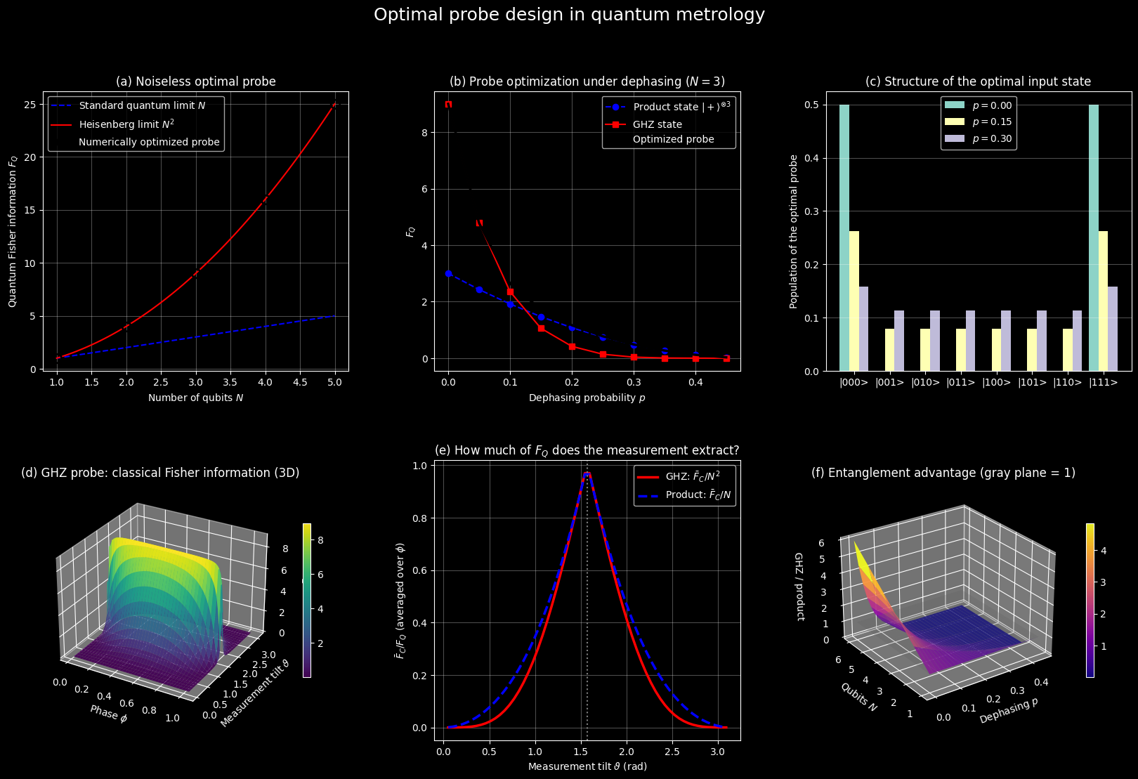
- (A) For $N=1,\dots,5$ the code optimizes over all pure states and compares the result with $N$ and $N^2$.
- (B) For $N=3$ and ten values of $p$ it compares the product state, GHZ and the numerically optimized probe.
- (C) It sweeps the measurement tilt $\vartheta$ and the phase $\varphi$ on a $60\times80$ grid. The phase range $0<\varphi<\pi/3$ covers one period of the GHZ signal $\cos 3\varphi$. The grids are offset slightly so they avoid the exact points where outcome probabilities vanish.
- (D) It evaluates the ratio $F_Q^{\rm GHZ}/F_Q^{\rm prod}$ for $N=1,\dots,6$ and 31 values of $p$. It also reports the largest deviation from the closed-form expressions, which serves as a built-in correctness check of
mixed_qfi.
The figure
All six panels are drawn in a single GridSpec figure. Panels (d) and (f) are 3D surfaces.
4. Results
=== (A) Noiseless case ===
  N   product       GHZ   optimized    N^2
  1    1.0000    1.0000      1.0000      1
  2    2.0000    4.0000      4.0000      4
  3    3.0000    9.0000      9.0000      9
  4    4.0000   16.0000     16.0000     16
  5    5.0000   25.0000     25.0000     25

=== (B) Local dephasing, N = 3 ===
     p   product       GHZ   optimized
 0.000    3.0000    9.0000      9.0000
 0.050    2.4300    4.7830      4.7830
 0.100    1.9200    2.3593      2.6425
 0.150    1.4700    1.0588      1.7240
 0.200    1.0800    0.4199      1.1678
 0.250    0.7500    0.1406      0.7770
 0.300    0.4800    0.0369      0.4867
 0.350    0.2700    0.0066      0.2711
 0.400    0.1200    0.0006      0.1201
 0.450    0.0300    0.0000      0.0300

=== (C) Measurement ===
GHZ, computational-basis-like tilt (theta ~ 0): mean F_C = 0.0000
GHZ, near-equatorial tilt (theta ~ pi/2):       mean F_C = 8.7309  (F_Q = 9)
Product, near-equatorial tilt (theta ~ pi/2):   mean F_C = 2.8973  (F_Q = 3)

=== (D) Closed-form check ===
max |numerical - analytic| over the (N, p) grid = 2.13e-14
N = 3: GHZ stops beating the product state near p = 0.1201
Total computation time: 2.1 s
5. Discussion of the Results
(a) Noiseless optimum: the Heisenberg limit emerges from the optimizer
The black circles are the best QFI values found by the optimizer for $N=1,\dots,5$. They sit on the red curve $N^2$ and well above the blue line $N$. The optimizer started from random states and was never told about GHZ, yet it reproduced the bound $F_Q\le(g_{\max}-g_{\min})^2=N^2$. For $N=3$ the values are $3$ for the product state and $9$ for both GHZ and the optimized probe.
(b) Under dephasing, GHZ is not always best
At $p=0$ the optimized probe equals GHZ ($F_Q=9$). GHZ coherence decays as $(1-2p)^{N}$, so its QFI collapses like $(1-2p)^{2N}$ while the product state’s QFI decays only like $(1-2p)^2$. The curves cross near $p\approx0.12$. In the intermediate regime ($p\approx0.1$–$0.3$) the optimized probe is strictly better than both reference states. At $p=0.10$, for example, the optimized value is about $2.64$, against roughly $2.36$ for GHZ and $1.92$ for the product state. For very large $p$ the optimum merges with the product state. No fixed textbook state is optimal across the whole range, which is the point of probe optimization.
(c) Structure of the optimal state
At $p=0$ the optimizer produces a GHZ state, with weight $0.5$ on $|000\rangle$ and $|111\rangle$ and nothing elsewhere. As noise grows, population leaks into the other six basis states. The weight on the two extreme states drops while the rest rises toward a uniform distribution, which is the signature of a product state $|+\rangle^{\otimes3}$ (every population equal to $1/8$). The optimal probe therefore interpolates between GHZ and a product state, shifting toward the more robust end as noise increases.
(d) 3D view: the measurement matters as much as the state
This surface shows the classical Fisher information $F_C(\varphi,\vartheta)$ of the GHZ probe. Near $\vartheta=\pi/2$, the $x$-basis, there is a high plateau close to $F_Q=9$. As $\vartheta\to0$ or $\pi$ the surface falls to zero. In the computational basis the outcome statistics of a GHZ state do not depend on $\varphi$ at all, so a perfect probe combined with the wrong measurement carries no information. The dips at the edges of the plateau, near $\varphi\to0$ and $\varphi\to\pi/3$, appear because some outcome probabilities approach zero there.
(e) How much of the QFI the measurement extracts
Averaged over $\varphi$, both the GHZ and product curves peak near $\vartheta=\pi/2$ at roughly $0.9$–$1.0$ of their respective $F_Q$. The GHZ curve is narrower, so entangled probes demand more precise measurement alignment. Entanglement raises the achievable sensitivity but makes it more fragile with respect to measurement errors.
(f) 3D view: where entanglement pays off
The surface is the ratio $F_Q^{\rm GHZ}/F_Q^{\rm prod}=N(1-2p)^{2N-2}$, and the gray plane marks ratio $=1$. In the noiseless limit the ratio equals $N$, so it grows linearly with the number of qubits. For any $p>0$ the exponent $2N-2$ makes larger GHZ states lose their advantage faster. The surface drops below the plane in a region that expands as $N$ increases, so the best probe size depends on the noise level. The console check confirms that the numerical QFI agrees with the closed forms to machine precision.
6. Takeaways
- The QFI bounds the best possible precision, so maximizing it over input states is the first step of probe design. In the noiseless case this gives the Heisenberg-limited GHZ state.
- The measurement must be matched to the probe. A GHZ state read out in the computational basis yields $F_C=0$, while an $x$-basis readout approaches $F_Q$.
- With noise, the optimal state is neither GHZ nor a product state. It is a numerically found compromise, and a short gradient-based optimization over $2^N$ amplitudes is enough to locate it.
- The same pipeline carries over to other generators, noise channels and qubit numbers. Only
generator_diaganddephasing_kernelneed to change.