How Much Better Can Entanglement Do? A Worked CHSH Example in Python
Two players, Alice and Bob, are placed in separate rooms and cannot communicate. A referee sends each of them a question, and each returns an answer. Together they win or lose according to a fixed rule. If they are allowed to share an entangled quantum state, how high can their winning probability go?
That number is the quantum value of the nonlocal game:
$$
\omega^*(G)=\sup_{|\psi\rangle,;{M^x_a},;{N^y_b}};\sum_{x,y}\pi(x,y)\sum_{a,b}V(a,b\mid x,y),\langle\psi|,M^x_a\otimes N^y_b,|\psi\rangle
$$
Here $\pi(x,y)$ is the question distribution, $V(a,b\mid x,y)\in{0,1}$ is the winning predicate, and the supremum runs over all shared states and all local measurements.
In this post we compute it for the most famous example, the CHSH game, in three independent ways: an analytic strategy, a numerical see-saw optimisation, and a Monte Carlo simulation of the game itself.
1. The CHSH game
The referee draws two uniformly random bits $x,y\in{0,1}$ and sends $x$ to Alice and $y$ to Bob. They reply with bits $a$ and $b$. They win if and only if
$$
a\oplus b ;=; x\wedge y .
$$
In words: the answers must be equal unless both questions are $1$, in which case they must differ.
Classical value. Any shared randomness is a mixture of deterministic strategies, so it suffices to check the $2^4=16$ deterministic ones. Winning all four question pairs would require $a_0\oplus b_0=0$, $a_0\oplus b_1=0$, $a_1\oplus b_0=0$ and $a_1\oplus b_1=1$. Adding the four equations modulo 2 gives $0=1$, which is a contradiction. At most three of the four can hold, so
$$
\omega_{\text{classical}}=\frac34 .
$$
Quantum value. With $\pm1$-valued observables $A_x,B_y$, the winning probability becomes
$$
P_{\text{win}}=\frac14\sum_{x,y}\frac{1+(-1)^{xy}\langle A_x\otimes B_y\rangle}{2}
=\frac12+\frac{S}{8},
$$
where
$$
S=\langle A_0B_0\rangle+\langle A_0B_1\rangle+\langle A_1B_0\rangle-\langle A_1B_1\rangle .
$$
Classically $|S|\le 2$, which reproduces $3/4$. Quantum mechanically, Tsirelson’s bound gives $|S|\le 2\sqrt2$, so
$$
\omega^*(\mathrm{CHSH})=\frac12+\frac{2\sqrt2}{8}=\cos^2!\left(\frac{\pi}{8}\right)\approx 0.853553 .
$$
The no-signalling value is $1$, so the game separates three regimes: $0.75<0.8536<1$.
An explicit optimal strategy
Take the Bell state $|\Phi^+\rangle=\frac{1}{\sqrt2}(|00\rangle+|11\rangle)$ and the observables
$$
A(\theta)=\cos\theta,Z+\sin\theta,X .
$$
On $|\Phi^+\rangle$ we have $\langle Z\otimes Z\rangle=\langle X\otimes X\rangle=1$ and $\langle Z\otimes X\rangle=\langle X\otimes Z\rangle=0$, hence
$$
\langle\Phi^+|A(\alpha)\otimes A(\beta)|\Phi^+\rangle=\cos(\alpha-\beta).
$$
Choosing $\alpha_0=0,\ \alpha_1=\pi/2,\ \beta_0=\pi/4,\ \beta_1=-\pi/4$ gives each of the four correlators magnitude $\tfrac{\sqrt2}{2}$ with exactly the right signs, so $S=2\sqrt2$.
Without assuming the strategy: the see-saw method
The explicit strategy shows that $\cos^2(\pi/8)$ is achievable. To check that a generic optimiser also finds nothing better, we use a see-saw iteration in local dimension $d$. Define the Bell operator
$$
W=\sum_{x,y}(-1)^{xy},A_x\otimes B_y .
$$
The iteration repeats three exactly solvable steps:
- State step. For fixed observables, the best state is the eigenvector of $W$ with the largest eigenvalue $\lambda_{\max}$.
- Alice step. For a fixed state and fixed $B_y$, maximise $\operatorname{Tr}(A_xM_x)$ over $\pm1$-valued observables, where $M_x$ is obtained by partially tracing out Bob. The solution is $A_x=\operatorname{sign}!\big(\tfrac{M_x+M_x^\dagger}{2}\big)$.
- Bob step. The same as above with the roles exchanged.
Each step can only increase the value, so the winning probability $\tfrac12+\tfrac{\lambda}{8}$ rises monotonically and converges to a local optimum.
2. The complete source code
Everything is in a single cell.
1 | import itertools |
3. Code walkthrough
Section 1–2: the game and the classical value
win_pred(a, b, x, y) is the winning predicate $a\oplus b=x\wedge y$ written with Python’s bitwise operators. classical_value() enumerates all $2^4=16$ deterministic strategies $(a_0,a_1,b_0,b_1)$, counts how many of the four question pairs each one wins, and keeps the best fraction. Deterministic strategies are enough because any classical strategy using shared randomness is a convex combination of them. The result is exactly $3/4$.
Section 3: the explicit quantum strategy
obs(theta)builds the $\pm1$-valued observable $A(\theta)=\cos\theta,Z+\sin\theta,X$, a measurement along a direction in the $x$–$z$ plane of the Bloch sphere.phi_plusis the Bell state $|\Phi^+\rangle$ as a four-component vector.win_probabilityevaluates $\tfrac14\sum_{x,y}\tfrac{1+(-1)^{xy}\langle A_x\otimes B_y\rangle}{2}$ literally, usingnp.kronfor the tensor product. It serves as the reference implementation.win_probability_fastuses the closed form $\langle A(\alpha)\otimes A(\beta)\rangle=\cos(\alpha-\beta)$, so the entire expression is a sum of four cosines. It accepts NumPy arrays, which matters in Section 7.
alpha_opt and beta_opt store the optimal angles derived above.
Section 4: the see-saw
sign_operator(M)takes the Hermitian part of $M$, diagonalises it, and replaces each eigenvalue by $+1$ or $-1$ according to its sign. This is the matrix sign function and gives the best $\pm1$-valued observable for a linear objective $\operatorname{Tr}(AM)$.random_observable(d, rng)produces a random starting point by applyingsign_operatorto a random complex matrix.- Inside
seesaw, the state is reshaped into a four-index tensorrho[a, b, a', b']. Theeinsumcalls contract this tensor with Bob’s observable (or Alice’s) to give the effective operator $M_x$ (or $M_y$) acting on the other party’s system. The result is passed tosign_operator. - After each full sweep, the Bell operator’s expectation value is converted to a winning probability $\tfrac12+\tfrac{\lambda}{8}$ and appended to
history.
The state is found as the top eigenvector of a $d^2\times d^2$ matrix, so for $d=2,3$ the whole optimisation takes a fraction of a second. Using local dimension $d=3$ lets the optimiser use strategies beyond qubits. The fact that it does not exceed $\cos^2(\pi/8)$ is consistent with Tsirelson’s theorem.
Section 5: Monte Carlo simulation
This section plays the game rather than computing an expectation. First, for each of the four question pairs, the exact joint outcome distribution $p(a,b\mid x,y)=\langle\Phi^+|P^x_a\otimes P^y_b|\Phi^+\rangle$ is computed from the projectors $P=\tfrac{I\pm A}{2}$. Then 200,000 question pairs are sampled.
Speed-up. A naive implementation would loop over rounds and sample one outcome per round, which is slow in pure Python. Here the rounds are grouped by question pair, and all the outcomes for each group are drawn with a single vectorised rng.choice call. The final running average is computed with np.cumsum. Only four sampling calls are needed instead of 200,000.
Section 6: running everything
The first block prints the classical, explicit quantum, analytic and no-signalling values. The see-saw is then run from 8 random starts in each of $d=2$ and $d=3$, and the best final values are printed. Finally the Monte Carlo game is run and its win rate is printed. Random starts are used because see-saw only guarantees a local optimum, and several restarts guard against a poor one.
Section 7: the figure
Speed-up for the 3D surface. Evaluating the winning probability on a $160\times160$ grid with win_probability would require 25,600 calls with four np.kron multiplications each. Instead, win_probability_fast accepts the whole meshgrid and returns the full surface in one vectorised expression.
4. Results as graphs
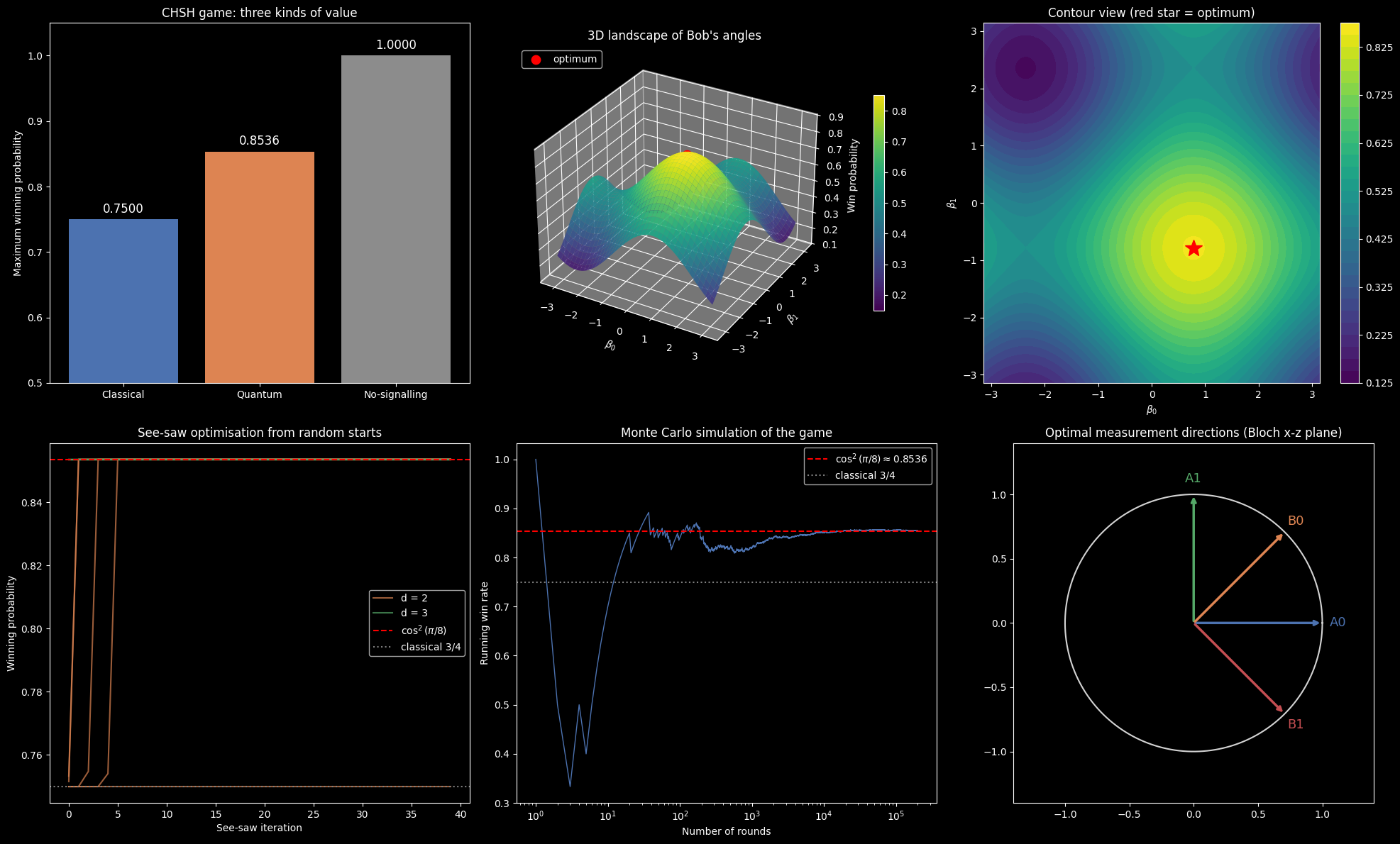
The six panels are in one figure.
How to read each panel
Panel 1, three kinds of value. The bars show $0.75$ (classical), $\cos^2(\pi/8)\approx0.8536$ (quantum) and $1$ (no-signalling). Entanglement gives a real, measurable advantage, but it stops well short of what an unrestricted no-signalling resource would allow.
Panel 2, 3D landscape. With Alice fixed at $\alpha_0=0,\ \alpha_1=\pi/2$, the surface shows Bob’s winning probability as a function of his two angles $(\beta_0,\beta_1)$. It is a smooth, periodic landscape with several peaks, and the red point marks the global maximum at $(\pi/4,-\pi/4)$ with height $\cos^2(\pi/8)$. The surface never rises above that point, which is Tsirelson’s bound in geometric form.
Panel 3, contour view. The same surface seen from above. The red star sits at the center of the brightest region, and the symmetric pattern of ridges reflects the cosine structure $\cos(\alpha-\beta)$.
Panel 4, see-saw convergence. Each curve is one random start. Every curve increases monotonically, as the theory guarantees, and the curves for both $d=2$ and $d=3$ settle at the red dashed line $\cos^2(\pi/8)$ and never cross it. Some starts get there in a few iterations; others pause on a plateau first. This is numerical evidence that the explicit qubit strategy is optimal even when more general strategies are allowed.
Panel 5, Monte Carlo. The running win rate of the simulated game fluctuates strongly for the first few hundred rounds and then converges toward the red dashed line. The log-scaled horizontal axis makes the $1/\sqrt{n}$ shrinkage of the fluctuations visible. The long-run rate clearly lies above the gray classical line at $3/4$, so no classical strategy could explain it.
Panel 6, optimal directions. The four arrows show the measurement axes of the optimal strategy in the Bloch $x$–$z$ plane. Alice’s axes ($A_0,A_1$) are orthogonal, and Bob’s axes ($B_0,B_1$) are orthogonal to each other and lie exactly halfway between Alice’s two axes. This symmetric picture is the geometric heart of the strategy: each of Bob’s axes is only $45^\circ$ away from both of Alice’s, which makes three of the four correlations as strong as possible, while the fourth is tuned to carry the required minus sign.
5. Console output
Classical value            : 0.75
Quantum value (explicit)   : 0.8535533906
cos^2(pi/8) (analytic)     : 0.8535533906
No-signalling value        : 1.0
See-saw best (d=2)         : 0.85355339
See-saw best (d=3)         : 0.85355339
Monte Carlo win rate       : 0.85456 (200000 rounds)
How to read the numbers
- Classical value is exactly $3/4$, in agreement with the argument that no deterministic strategy wins all four question pairs.
- Quantum value (explicit) and $\cos^2(\pi/8)$ agree to ten digits, confirming the analytic derivation.
- See-saw best for $d=2$ and $d=3$ both match $\cos^2(\pi/8)$ to the printed precision. Higher local dimension did not help.
- Monte Carlo win rate is close to $0.8536$. With $n=200{,}000$ rounds the statistical standard deviation is about $\sqrt{p(1-p)/n}\approx 0.0008$, so deviations in the third decimal place are expected.
6. Wrap-up
The quantum value of a nonlocal game is the best winning probability over all entangled strategies. For the CHSH game it equals
$$
\omega^*(\mathrm{CHSH})=\cos^2!\left(\frac{\pi}{8}\right)=\frac12+\frac{\sqrt2}{4}\approx 0.8536 ,
$$
compared with $3/4$ classically. The explicit Bell-state strategy reaches this value, the see-saw optimisation finds nothing better, and a simulation of the game confirms it empirically. For general games the exact quantum value is hard to compute, but see-saw gives lower bounds, and semidefinite hierarchies such as the NPA hierarchy give matching upper bounds. Try changing the winning predicate or the question distribution in the code and see how the three values move.