Minimizing Relative Entropy and Robustness
How entangled is a quantum state? A yes/no answer (separable or entangled) is not enough for most purposes. We want a number. Many entanglement measures are defined as the minimum “distance” from the given state to the set of separable states. In this post we compute two of them numerically for two-qubit states:
- the relative entropy of entanglement (a nonconvex optimization over separable states), and
- the generalized robustness of entanglement (a semidefinite program).
We check both against exact formulas and visualize them over a two-parameter family of states, including 3D surfaces.
1. The Measures
Let $\mathrm{SEP}$ denote the set of separable states. A state is separable if it can be written as
$$
\sigma = \sum_k p_k, |a_k\rangle\langle a_k| \otimes |b_k\rangle\langle b_k| ,\qquad p_k\ge 0,\ \sum_k p_k = 1 .
$$
Relative entropy of entanglement
$$
E_R(\rho) = \min_{\sigma\in \mathrm{SEP}} S(\rho,|,\sigma),\qquad
S(\rho|\sigma) = \mathrm{Tr}\left[\rho\left(\log_2\rho - \log_2\sigma\right)\right].
$$
Generalized robustness of entanglement

This is the minimum amount of “noise” $\tau$ that must be mixed in to destroy the entanglement. Setting $Y=(1+s)\sigma$ turns it into a semidefinite program (SDP):
$$
R_G(\rho)=\min_{Y}\ \mathrm{Tr},Y - 1\quad \text{s.t.}\quad Y\succeq \rho,\quad Y^{T_B}\succeq 0 .
$$
For two qubits, “separable” is equivalent to “positive partial transpose” (the Peres–Horodecki criterion). This is why the constraint $Y^{T_B}\succeq 0$ is exact here.
The inequality connecting them
The log-robustness upper-bounds the relative entropy of entanglement:
$$
E_R(\rho)\ \le\ \log_2\bigl(1+R_G(\rho)\bigr).
$$
2. The Example Problem
Problem 1 (Werner states).
$$
\rho_W(p) = p,|\Phi^+\rangle\langle\Phi^+| + (1-p)\frac{I}{4},\qquad |\Phi^+\rangle=\frac{|00\rangle+|11\rangle}{\sqrt2}.
$$
With the singlet fraction $F=\langle\Phi^+|\rho_W|\Phi^+\rangle=\frac{3p+1}{4}$, the exact results for $F>1/2$ (that is, $p>1/3$) are
$$
E_R = 1 - h(F),\qquad h(x)=-x\log_2 x-(1-x)\log_2(1-x),\qquad R_G = 2F-1 = \frac{3p-1}{2},
$$
and both vanish for $p\le 1/3$. We recover these numerically.
Problem 2 (two-parameter family).
$$
\rho(p,\theta) = p,|\psi_\theta\rangle\langle\psi_\theta| + (1-p)\frac{I}{4},\qquad |\psi_\theta\rangle=\cos\theta,|00\rangle+\sin\theta,|11\rangle .
$$
The partial transpose has smallest eigenvalue $\frac{1-p}{4}-\frac{p\sin 2\theta}{2}$, so the state is separable exactly when
$$
p\le \frac{1}{1+2\sin 2\theta}.
$$
For pure states ($p=1$), the exact values are $E_R=h(\cos^2\theta)$ (the entanglement entropy) and $R_G=\sin 2\theta$.
We compute $E_R$ and $R_G$ on a $(p,\theta)$ grid and draw 3D surfaces.
3. Numerical Strategy
Relative entropy. The set $\mathrm{SEP}$ is hard to describe directly, so we parametrize it from the inside. We write
$$
\sigma(\mathbf{x}) = \sum_{k=1}^{K} p_k, |a_k b_k\rangle\langle a_k b_k|,\qquad
p_k=\frac{e^{\ell_k}}{\sum_j e^{\ell_j}},\qquad
|a\rangle=\begin{pmatrix}\cos\frac{\vartheta}{2}\ e^{i\varphi}\sin\frac{\vartheta}{2}\end{pmatrix}.
$$
This $\sigma$ is separable for every parameter value, so minimizing $S(\rho|\sigma(\mathbf x))$ with L-BFGS-B gives an upper bound on $E_R$ that converges to the true value as the optimizer converges. We use $K=8$ product states and several random restarts.
Robustness. This is a convex SDP, so we hand it to CVXPY.
4. Source Code
1 | import time |
5. Code Walkthrough
Basic tools
werner(p) and family(p, theta) build the $4\times4$ density matrices. partial_transpose reshapes $\rho$ into a rank-4 tensor $\rho_{i j, k l}\to\rho_{i,l,,k,j}$ by swapping the two indices of the second qubit, which is the partial transpose $T_B$. negativity sums the absolute values of the negative eigenvalues of $\rho^{T_B}$. binary_entropy is clipped away from $0$ and $1$ so that the $\log$ never produces nan.
Parametrizing separable states
build_sigma maps a flat parameter vector $\mathbf x\in\mathbb R^{5K}$ to a separable density matrix:
- The first $K$ entries are logits. A softmax (shifted by the maximum for numerical stability) turns them into probabilities $p_k$, so positivity and normalization hold automatically and the problem becomes unconstrained.
- The remaining $4K$ entries are Bloch-sphere angles $(\vartheta_A,\varphi_A,\vartheta_B,\varphi_B)$ for each term.
- The vectors $|a_k\rangle$ and $|b_k\rangle$ are built for all $k$ at once. The batched outer product
A[:, :, None] * B[:, None, :]gives all $K$ product vectors $|a_kb_k\rangle$ in one operation. - A single
einsumassembles $\sigma=\sum_k p_k|\psi_k\rangle\langle\psi_k|$.
Because every $\sigma$ produced this way is separable, the optimizer can never wander outside $\mathrm{SEP}$.
Objective function
Since $S(\rho|\sigma)=\mathrm{Tr},\rho\log_2\rho-\mathrm{Tr},\rho\log_2\sigma$, the first term is a constant, computed once in make_objective. Each evaluation only diagonalizes $\sigma$ once: eigh gives $\sigma=V,\mathrm{diag}(w),V^\dagger$, and $\log_2\sigma=V,\mathrm{diag}(\log_2 w),V^\dagger$. The eigenvalues are clipped at $10^{-13}$ so that a numerically zero eigenvalue cannot produce -inf. The term (V * lw) @ V.conj().T multiplies column-wise by lw, which avoids building a diagonal matrix.
Optimization and speed-ups
The landscape is nonconvex in $\mathbf x$, so relative_entropy_of_entanglement runs L-BFGS-B from several random starts and keeps the best. The code is already in its accelerated form, and four design choices keep the runtime to roughly a minute or so on a standard CPU:
- The objective has no Python loops over the $K$ product states (batched arrays and
einsum). - Only one $4\times4$ eigendecomposition is needed per evaluation.
- On the $(p,\theta)$ grid, the optimum found for the previous $p$ is passed as a warm start (
x0=x_prev) for the next one, so only 2 random restarts are needed there. - The robustness problem is a tiny convex SDP, solved in about 10–20 ms per state.
Robustness SDP
generalized_robustness is a direct translation of the SDP above. Because all of our states are real, the optimal $Y$ can be taken to be real symmetric (averaging a solution with its complex conjugate keeps it feasible and optimal), so symmetric=True suffices and keeps the problem small. The constraint Y - rho_r >> 0 encodes $Y\succeq\rho$, and cp.partial_transpose(Y, dims=[2, 2], axis=1) >> 0 encodes $Y^{T_B}\succeq0$. The objective $\mathrm{Tr},Y-1$ equals $s$.
Experiments
Part (3) sweeps 13 values of the Werner parameter $p$ and compares numerical results with the exact formulas $E_R=1-h(F)$ and $R_G=2F-1$. Part (4) evaluates both measures on an $11\times 9$ grid in $(p,\theta)$, and checks the pure-state values at $p=1$ and the inequality $E_R\le\log_2(1+R_G)$.
Plotting
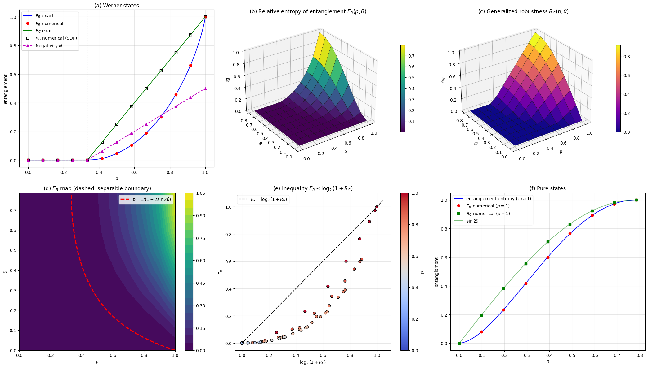
All six panels live in one figure. Panels (b) and (c) are 3D surfaces created with projection="3d". The legends and axis labels use TeX syntax in raw strings.
6. Execution Results
=== Werner states: rho = p|Phi+><Phi+| + (1-p) I/4 ===
     p       F   E_R(num)  E_R(exact)   R_G(num)  R_G(exact)       N
 0.000  0.2500   0.000000    0.000000   0.000000    0.000000  0.0000
 0.083  0.3125   0.000000    0.000000   0.000000    0.000000  0.0000
 0.167  0.3750   0.000000    0.000000   0.000000    0.000000  0.0000
 0.250  0.4375   0.000000    0.000000   0.000000    0.000000  0.0000
 0.333  0.5000   0.000000    0.000000   0.000000    0.000000  0.0000
 0.417  0.5625   0.011301    0.011301   0.125000    0.125000  0.0625
 0.500  0.6250   0.045566    0.045566   0.250000    0.250000  0.1250
 0.583  0.6875   0.103962    0.103962   0.375000    0.375000  0.1875
 0.667  0.7500   0.188722    0.188722   0.500000    0.500000  0.2500
 0.750  0.8125   0.303788    0.303788   0.625000    0.625000  0.3125
 0.833  0.8750   0.456436    0.456436   0.750000    0.750000  0.3750
 0.917  0.9375   0.662710    0.662710   0.875000    0.875000  0.4375
 1.000  1.0000   1.000000    1.000000   1.000000    1.000000  0.5000
max |E_R(num) - E_R(exact)| = 6.45e-08
max |R_G(num) - R_G(exact)| = 3.37e-09

=== Pure states (p = 1): E_R vs. entanglement entropy ===
theta = 0.0000   E_R(num) = 0.000000   entropy = 0.000000
theta = 0.0982   E_R(num) = 0.078179   entropy = 0.078179
theta = 0.1963   E_R(num) = 0.233327   entropy = 0.233327
theta = 0.2945   E_R(num) = 0.417032   entropy = 0.417032
theta = 0.3927   E_R(num) = 0.600876   entropy = 0.600876
theta = 0.4909   E_R(num) = 0.764191   entropy = 0.764191
theta = 0.5890   E_R(num) = 0.891619   entropy = 0.891619
theta = 0.6872   E_R(num) = 0.972369   entropy = 0.972368
theta = 0.7854   E_R(num) = 1.000000   entropy = 1.000000

max over grid of [E_R - log2(1+R_G)] = 6.28e-08  (<= 0 up to numerical tolerance)
Total computation time: 157.6 s
7. Discussion of the Results
Console output
The Werner table shows that the optimization over separable states reproduces the exact result. In my run the maximum deviation was about $6\times10^{-8}$ for $E_R$ and about $3\times10^{-9}$ for $R_G$. Some concrete values:
| $p$ | $F$ | $E_R$ | $R_G$ |
|---|---|---|---|
| $0.333$ | $0.5000$ | $0$ | $0$ |
| $0.500$ | $0.6250$ | $0.045566$ | $0.2500$ |
| $0.750$ | $0.8125$ | $0.303788$ | $0.6250$ |
| $1.000$ | $1.0000$ | $1.0000$ | $1.0000$ |
Both measures vanish for $p\le 1/3$ and become positive immediately afterward, which is the Peres–Horodecki threshold $F=1/2$. The pure-state table shows that $E_R$ matches the entanglement entropy $h(\cos^2\theta)$ to about six digits at every $\theta$. Finally, $\max[E_R-\log_2(1+R_G)]$ is of order $10^{-8}$, which is zero up to numerical tolerance (it is not exactly nonpositive because the optimizer stops at a finite tolerance). The inequality holds everywhere, with equality at the maximally entangled state.
Panel (a): Werner states
Red dots ($E_R$ from the optimizer) lie on the blue curve ($1-h(F)$). Black squares ($R_G$ from the SDP) lie on the green line $2F-1$. Both are zero up to the dotted line at $p=1/3$. Note how different the shapes are: $R_G$ grows linearly in $p$ while $E_R$ grows slowly at first, like $(F-\tfrac12)^2$ near the threshold, and only catches up at $p=1$. The negativity (magenta) is exactly half of $R_G$ for these states, so it is a rescaled copy of the robustness. Different entanglement measures agree on which states are entangled but not on how much.
Panels (b) and (c): 3D surfaces
Both surfaces are flat at zero over a large region, the separable states, and rise toward the corner $p=1$, $\theta=\pi/4$, where the state is the maximally entangled Bell state. At that corner $E_R=R_G=1$. Both surfaces are monotonic in $p$ and in $\theta$, as expected: more purity and a more balanced Schmidt decomposition give more entanglement. The robustness surface (c) is noticeably more “tent-like” and rises earlier, whereas the relative-entropy surface (b) stays low over most of the domain and shoots up near $p\to1$. This is the same linear-versus-quadratic difference seen in panel (a).
Panel (d): the entanglement map
This is a top-down view of surface (b). The dashed red curve is the analytic boundary $p=1/(1+2\sin2\theta)$, which separates separable states (below and to the left) from entangled ones. The boundary passes through $p=1/3$ at $\theta=\pi/4$ (the Werner case) and reaches $p=1$ at $\theta=0$, where the pure state is a product state. The region where $E_R$ is exactly zero coincides with this analytic boundary, which confirms that the numerical optimizer correctly detects the transition.
Panel (e): the inequality $E_R\le\log_2(1+R_G)$
Each dot is one grid state, coloured by $p$. All dots lie on or below the dashed diagonal, which is the bound $E_R\le\log_2(1+R_G)$. The points touch the diagonal only at the origin (separable states) and at the Bell state (top right). Mixed states and partially entangled pure states sit strictly below it. The gap shows that the two measures encode genuinely different information about the state.
Panel (f): pure states
For pure states, the numerical $E_R$ (red dots) matches the entanglement entropy $h(\cos^2\theta)$ (blue curve), as it must, since for pure states the closest separable state is the dephased state. The numerical $R_G$ (green squares) lies on $\sin2\theta$, in agreement with the closed form $(\sum_i\sqrt{\lambda_i})^2-1$ for pure states with Schmidt coefficients $\lambda_i$. Here $\sin 2\theta\ge h(\cos^2\theta)$ for all $\theta$, again consistent with $E_R\le\log_2(1+R_G)$.
8. Summary
- Distance-based entanglement measures reduce to optimization problems: a nonconvex one for the relative entropy and a convex SDP for the robustness.
- Parametrizing separable states from the inside (softmax weights times Bloch-sphere product states) turns the constrained problem into an unconstrained one that L-BFGS-B handles quickly.
- Vectorization, a single eigendecomposition per evaluation, and warm starts keep the full 3D study down to about a minute or so.
- The numerical results match the exact Werner, pure-state and PPT-boundary formulas to $10^{-7}$ or better, and they confirm $E_R\le\log_2(1+R_G)$.
The same approach extends to other measures, such as the geometric measure, by changing the objective, and to higher-dimensional systems, where PPT is only a relaxation of separability and the inner parametrization used here becomes the more reliable route.