Finding the Channel That Maximizes Fidelity with Python
The no-cloning theorem says that no physical process can turn an unknown quantum state $|\psi\rangle$ into $|\psi\rangle\otimes|\psi\rangle$ exactly. It does not forbid approximate copies. If we accept imperfect copies, the natural question is how good they can be. This article answers that for a qubit by treating the cloner as a convex optimization problem over quantum channels, and then solving a concrete instance numerically.
1. The Problem
A $1\to 2$ cloning machine is a completely positive trace-preserving (CPTP) map
$$
\Lambda:\ \mathcal{L}(\mathbb{C}^2)\ \to\ \mathcal{L}(\mathbb{C}^2\otimes\mathbb{C}^2),
$$
taking one input qubit to two output qubits, $A$ and $B$. For a pure input $|\psi\rangle$, the single-copy fidelities are
$$
F_A(\psi)=\langle\psi|,\mathrm{Tr}_B,\Lambda(|\psi\rangle\langle\psi|),|\psi\rangle,\qquad
F_B(\psi)=\langle\psi|,\mathrm{Tr}_A,\Lambda(|\psi\rangle\langle\psi|),|\psi\rangle .
$$
We want a universal cloner that works equally well for every input state, so we maximize the average over the Haar measure on pure states:
$$
\bar F_\lambda(\Lambda)=\int d\psi,\Big[\lambda,F_A(\psi)+(1-\lambda),F_B(\psi)\Big],\qquad \lambda\in[0,1].
$$
The symmetric case $\lambda=\tfrac12$ is the classic Bužek–Hillery problem. Other values of $\lambda$ give asymmetric cloners, which trade quality of copy $A$ against copy $B$.
Known analytic answer (our benchmark)
For $\lambda=\tfrac12$ the optimum is
$$
F_{\mathrm{opt}}=\frac56\approx 0.8333,
$$
reached by the transformation
$$
|0\rangle\ \mapsto\ \sqrt{\tfrac23},|00\rangle|\uparrow\rangle+\sqrt{\tfrac13},|\Psi^+\rangle|\downarrow\rangle,\qquad
|\Psi^+\rangle=\tfrac{1}{\sqrt2}(|01\rangle+|10\rangle),
$$
together with its mirror image for $|1\rangle$. Each output qubit’s Bloch vector is shrunk by the factor $\eta=2F-1=\tfrac23$.
We will not hard-code this. We solve the optimization numerically and check that it rediscovers $5/6$, then map the whole asymmetric trade-off curve.
2. Turning the Problem into Linear Algebra
Stinespring form
Every channel $\Lambda$ can be written as an isometry $V:\mathbb{C}^2\to\mathbb{C}^2_A\otimes\mathbb{C}^2_B\otimes\mathbb{C}^{r}_E$ followed by a partial trace over the environment $E$:
$$
\Lambda(\rho)=\mathrm{Tr}_E!\left[V\rho V^\dagger\right],\qquad V^\dagger V=\mathbb{1}_2 .
$$
The Choi rank of a map from $\mathbb{C}^2$ to $\mathbb{C}^4$ is at most $8$, so $r=8$ covers every possible cloner.
Replacing the Haar integral by six states
With $P_\psi=|\psi\rangle\langle\psi|$, the fidelity is
$$
F_A(\psi)=\mathrm{Tr}!\left[\big(P_\psi\otimes\mathbb{1}_B\otimes\mathbb{1}_E\big),V P_\psi V^\dagger\right],
$$
which is a degree-2 polynomial in $P_\psi$. The six states at the vertices of the Bloch-sphere octahedron ($\pm x,\pm y,\pm z$) form a projective 2-design. The Haar average of any such polynomial therefore equals the plain average over these six states, exactly:
$$
\bar F_\lambda(V)=\frac16\sum_{s=1}^{6}\mathrm{Tr}!\left[V^\dagger Q_s V R_s\right],
$$

A fast fixed-point algorithm
Because $Q_s\succeq0$ and $R_s\succeq0$, the objective is a convex quadratic form in $V$. Maximizing it over the set of isometries ${V^\dagger V=\mathbb{1}}$ can be done by a power-iteration-like scheme. Define the gradient matrix
$$
G(V)=\sum_{s=1}^{6}Q_s,V,R_s,
$$
and update with the polar factor of $G$. If $G=U\Sigma W^\dagger$ is a thin singular value decomposition, then
$$
V_{n+1}=U,W^\dagger .
$$
This choice maximizes $\mathrm{Re},\mathrm{Tr}(G^\dagger V)$ over all isometries. Convexity guarantees
$$
\bar F_\lambda(V_{n+1})\ \ge\ \bar F_\lambda(V_n),
$$
so the objective rises monotonically. Each iteration costs a few microseconds. No semidefinite-programming solver is needed, which is also the speed-up for this problem: a generic SDP or gradient solver would take far longer for the 21-point trade-off sweep.
3. Reference Strategies
We compare the optimized cloner against two simple strategies.
CNOT cloner. It maps $\alpha|0\rangle+\beta|1\rangle\mapsto\alpha|00\rangle+\beta|11\rangle$ and is not universal. Its fidelity depends on the input state:
$$
F(\theta)=1-\tfrac12\sin^2\theta,\qquad \bar F=\tfrac23 .
$$
Measure-and-prepare. Optimal state estimation from one copy gives
$$
\bar F=\tfrac23 .
$$
4. Full Source Code
1 | import numpy as np |
5. Code Walkthrough
Section 1 – Dimensions
The output space is two qubits, so DIM_OUT = 4. The environment dimension is R_ENV = 8, which is the largest Choi rank a map from $\mathbb{C}^2$ to $\mathbb{C}^4$ can have. The isometry $V$ is therefore a $32\times 2$ complex matrix. Its row index encodes $(a,b,e)$ as $(2a+b)\cdot 8+e$, which matches the Kronecker-product ordering used later.
Section 2 – The octahedron design
octa_states lists the six states $|\pm x\rangle,|\pm y\rangle,|\pm z\rangle$. R_list stores their projectors $R_s$. QA and QB hold $P_s\otimes\mathbb{1}\otimes\mathbb{1}$ and $\mathbb{1}\otimes P_s\otimes\mathbb{1}$, so that $Q_s=\lambda Q^A_s+(1-\lambda)Q^B_s$ can be formed for any weight with a single line of array arithmetic.
Section 3 – Core routines
polar_isometrycomputes $UW^\dagger$ from a thin SVD. It is the projection of an arbitrary matrix onto the nearest isometry.gradient_and_objectiveevaluates $G=\sum_s Q_sVR_s$ with oneeinsumcall and returns $\bar F=\frac16\mathrm{Re},\mathrm{Tr}(V^\dagger G)$.optimize_clonerruns the monotone iteration $V\leftarrow\mathrm{polar}(G(V))$ from several random isometries and keeps the best one. Random restarts guard against the possibility of non-global stationary points. The loop stops when the increase falls below $10^{-13}$.single_copy_fidelitiesis a fully vectorized fidelity evaluator. It uses the identity
$$
F_A(\psi)=\sum_{b,e}\Big|\sum_a \langle\psi|a\rangle,\Psi_{abe}\Big|^2,\qquad \Psi=V|\psi\rangle,
$$
which avoids building density matrices and handles thousands of states in one call. This function runs the Haar-random verification and the Bloch-sphere grid with no Python loops.
Section 4 – The CNOT cloner
The CNOT cloner is encoded as an isometry with a trivial environment: $|0\rangle\to|00\rangle$ sits at row $0$ and $|1\rangle\to|11\rangle$ at row $3\cdot R_{\mathrm{ENV}}$. It serves as a non-universal baseline evaluated with exactly the same machinery.
Section 5 – The symmetric optimum
With $\lambda=\tfrac12$ the optimizer is run from six random starts. The script then reports the following:
- the optimized average fidelity compared with $5/6$;
- the isometry defect $|V^\dagger V-\mathbb{1}|$, which verifies that the channel is trace preserving;
- the Bloch shrinking factor $\eta$ for the input $|0\rangle$, via $\rho_A=\mathrm{Tr}_{B,E}|\Psi\rangle\langle\Psi|$;
- the numerical Kraus rank, taken from the singular values of the matrix whose rows are the vectorized Kraus operators;
- a check against $20000$ Haar-random pure states, which confirms that the six-state average really equals the Haar average.
The theory predicts a Kraus rank of $2$, because the optimal cloner can be written as
$$
\Lambda(\rho)=\tfrac23,\Pi_{\mathrm{sym}}(\rho\otimes\mathbb{1})\Pi_{\mathrm{sym}},
$$
with $\Pi_{\mathrm{sym}}$ the projector onto the symmetric subspace of two qubits.
Section 6 – Asymmetric trade-off
The same optimizer is repeated for 21 weights $\lambda\in[0,1]$. At $\lambda=1$ the best strategy is to hand the input to $A$ untouched ($F_A=1$) and give $B$ only a maximally mixed qubit ($F_B=\tfrac12$). The intermediate weights trace out the Pareto frontier between the two copies.
Section 7 – Visualization
All six panels live in a single figure (see the next section for how to read it).
6. Execution Results
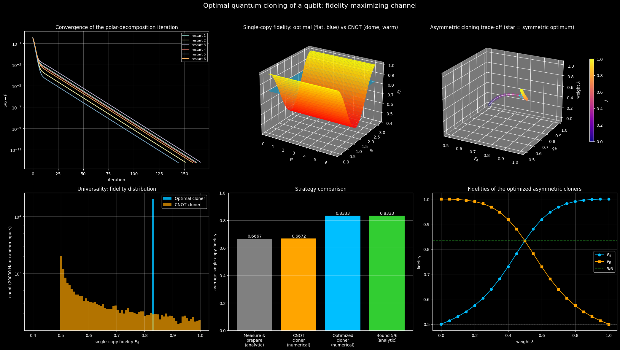
=== Symmetric optimal cloner (lambda = 0.5) ===
Optimized average fidelity      : 0.833333333333
Analytic optimum 5/6            : 0.833333333333
Absolute error                  : 6.052e-13
Isometry error ||V^dag V - I||  : 9.956e-16
F_A (octahedron average)        : 0.833333333333
F_B (octahedron average)        : 0.833333333333
Bloch shrinking factor eta      : 0.666664184649   (analytic 2/3 = 0.666666666667)
Numerical Kraus rank            : 2

=== Haar-random check with 20000 states ===
Optimal cloner : mean F_A = 0.833333322, mean F_B = 0.833333322, spread of F_A = 3.110e-06
CNOT cloner    : mean F_A = 0.667233172, min = 0.5000, max = 1.0000

=== Asymmetric trade-off (selected weights) ===
  lambda          F_A          F_B
    0.00   0.50000000   1.00000000
    0.25   0.60367259   0.98163706
    0.50   0.83333333   0.83333333
    0.75   0.98163706   0.60367259
    1.00   1.00000000   0.50000000
7. Reading the Results
Convergence (top left). The vertical axis is the gap $5/6-\bar F$ on a logarithmic scale. Because each update is a polar projection of the gradient of a convex quadratic form, every curve decreases monotonically. All restarts should approach the same floor near machine precision. That agreement is numerical evidence that the symmetric optimum is a global one and that the algorithm does not stall in spurious local maxima.
Fidelity over the Bloch sphere (top middle, 3D). The horizontal plane is the parameter space $(\varphi,\theta)$ of input states, and the height is $F_A$. The optimized cloner appears as a perfectly flat sheet at $5/6$: it copies every state equally well, which is exactly what universal means. The CNOT cloner forms a dome, $1-\tfrac12\sin^2\theta$. It is perfect at the poles ($|0\rangle$ and $|1\rangle$, the basis states it was designed for) and drops to $\tfrac12$ on the equator. Its average over the sphere is only $\tfrac23$. The flatness of the blue sheet is a numerical rediscovery of the covariance of the optimal channel, which the optimizer was never told to impose.
Trade-off curve (top right, 3D). Each point is one optimized cloner with $x=F_A$, $y=F_B$ and height equal to the weight $\lambda$. The curve runs from $(F_A,F_B)=(\tfrac12,1)$ at $\lambda=0$ to $(1,\tfrac12)$ at $\lambda=1$, and passes through the symmetric optimum $(\tfrac56,\tfrac56)$ marked by the star. Its concavity matters physically: improving one copy beyond $5/6$ always costs more than a one-for-one loss in the other, which is a quantitative form of the no-cloning theorem.
Fidelity histogram (bottom left). For 20000 Haar-random inputs, the optimal cloner puts essentially all of its weight in a single bin at $5/6$ (note the logarithmic vertical axis). The CNOT cloner is spread over $[\tfrac12,1]$. The spread, not just the mean, separates a universal machine from a basis-dependent one.
Strategy comparison (bottom middle). Measure-and-prepare and the CNOT cloner both give $\tfrac23$. The optimized quantum cloner reaches $\tfrac56$, which matches the analytic bound. Quantum-coherent copying beats the best classical strategy of measuring once and re-preparing.
Fidelities versus the weight (bottom right). $F_A$ rises and $F_B$ falls as $\lambda$ increases, and the curves cross at $\lambda=\tfrac12$ at the height $5/6$. They saturate at the extremes: $F_A=1$ means the second copy carries no information beyond a random guess of fidelity $\tfrac12$.
8. Summary
- Optimal approximate cloning is a convex quadratic maximization over isometries, which is a semidefinite program in disguise.
- Replacing the Haar integral with an exact 2-design (six octahedron states) reduces the problem to a few small matrix products.
- The fixed-point iteration $V\leftarrow\mathrm{polar}\big(\sum_s Q_sVR_s\big)$ increases the objective monotonically and recovers the Bužek–Hillery value $\bar F=5/6$, the shrinking factor $\eta=2/3$ and a Kraus rank of $2$, without any hand-built ansatz.
- The same code, with only the weight $\lambda$ changed, maps the whole asymmetric trade-off curve between the two copies.