Maximizing the Error-Free Success Probability
Introduction
Suppose someone hands you a qubit and tells you it is in one of two known pure states, $|\psi_1\rangle$ or $|\psi_2\rangle$. If the states are not orthogonal, no measurement can tell them apart perfectly. Two philosophies exist for dealing with this limitation:
- Minimum-error discrimination always gives an answer, but accepts that the answer is sometimes wrong. The optimum is given by the Helstrom bound.
- Unambiguous state discrimination (USD) never gives a wrong answer, but accepts that the measurement sometimes returns “I don’t know”. The goal is to maximize the probability of a conclusive and correct result.
USD is the right tool whenever a wrong answer is far more costly than no answer at all, as in quantum key distribution or quantum money verification. In this article we formulate USD as a small constrained optimization problem, derive the closed-form optimum, verify it by brute-force search, simulate the measurement with Monte Carlo sampling, and visualize everything, including 3D landscapes.
Problem Formulation
Let the two states be prepared with prior probabilities $\eta_1$ and $\eta_2 = 1-\eta_1$, and let their overlap be
$$
s = \langle \psi_1 | \psi_2 \rangle, \qquad 0 \le |s| < 1 .
$$
We look for a three-outcome POVM ${\Pi_1, \Pi_2, \Pi_?}$ with
$$
\Pi_1 + \Pi_2 + \Pi_? = I, \qquad \Pi_1,\Pi_2,\Pi_? \succeq 0 .
$$
Outcome “1” means “the state was $\psi_1$”, outcome “2” means “the state was $\psi_2$”, and outcome “?” means “inconclusive”. Error-free discrimination requires
$$
\langle \psi_2 | \Pi_1 | \psi_2 \rangle = 0, \qquad \langle \psi_1 | \Pi_2 | \psi_1 \rangle = 0 .
$$
The objective is the total probability of a conclusive result:
$$
P_{\mathrm{succ}} = \eta_1 \langle \psi_1 | \Pi_1 | \psi_1 \rangle + \eta_2 \langle \psi_2 | \Pi_2 | \psi_2 \rangle .
$$
The problem is therefore: maximize $P_{\mathrm{succ}}$ over POVMs subject to the zero-error constraints.
Reduction to a Two-Variable Optimization
The zero-error constraints force $\Pi_1$ to be proportional to the projector onto the vector orthogonal to $|\psi_2\rangle$, and $\Pi_2$ to be proportional to the projector onto the vector orthogonal to $|\psi_1\rangle$:
$$
\Pi_1 = p_1 |\psi_2^{\perp}\rangle\langle\psi_2^{\perp}|, \qquad
\Pi_2 = p_2 |\psi_1^{\perp}\rangle\langle\psi_1^{\perp}|, \qquad p_1,p_2 \in [0,1].
$$
Since $|\langle \psi_2^{\perp}|\psi_1\rangle|^2 = 1-|s|^2$, the objective becomes
$$
P_{\mathrm{succ}}(p_1,p_2) = (1-|s|^2),(\eta_1 p_1 + \eta_2 p_2).
$$
The remaining requirement is positivity of the inconclusive operator
$$
\Pi_? = I - p_1 |\psi_2^{\perp}\rangle\langle\psi_2^{\perp}| - p_2 |\psi_1^{\perp}\rangle\langle\psi_1^{\perp}| \succeq 0 .
$$
For a $2\times 2$ Hermitian matrix, positive semidefiniteness is equivalent to a non-negative trace and a non-negative determinant:
$$
\operatorname{tr}\Pi_? = 2 - p_1 - p_2 \ge 0, \qquad
\det \Pi_? = 1 - p_1 - p_2 + p_1 p_2 ,(1-|s|^2) \ge 0 .
$$
We have reduced the quantum problem to maximizing a linear function over a convex region in the $(p_1,p_2)$ plane.
Closed-Form Solution
Let $r = \sqrt{\eta_2/\eta_1}$. The optimum lies on the curve $\det\Pi_? = 0$, and solving the Lagrange conditions gives two regimes.
Regime I (moderate overlap), $|s| \le \min\left(r,, 1/r\right)$:
$$
p_1 = \frac{1 - r|s|}{1-|s|^2}, \qquad
p_2 = \frac{1 - |s|/r}{1-|s|^2}, \qquad
P_{\mathrm{succ}} = 1 - 2\sqrt{\eta_1\eta_2},|s| .
$$
Regime II (large overlap, strongly biased priors), $|s| > \min\left(r,,1/r\right)$. It is best to only identify the more probable state:
$$
P_{\mathrm{succ}} = \max(\eta_1,\eta_2),\bigl(1-|s|^2\bigr).
$$
For equal priors the answer simplifies to the famous Ivanovic–Dieks–Peres limit
$$
P_{\mathrm{succ}} = 1 - |\langle\psi_1|\psi_2\rangle| .
$$
For comparison, the minimum-error (Helstrom) success probability is
$$
P_{\mathrm{Hel}} = \frac{1}{2}\left(1 + \sqrt{1 - 4\eta_1\eta_2,|s|^2}\right),
$$
which is always larger than $P_{\mathrm{succ}}$. The difference is the price paid for certainty.
Concrete Example
We use two real qubit states in the plane,
$$
|\psi_1\rangle = \begin{pmatrix}1\0\end{pmatrix}, \qquad
|\psi_2\rangle = \begin{pmatrix}\cos\theta\ \sin\theta\end{pmatrix}, \qquad s = \cos\theta,
$$
and the orthogonal partners
$$
|\psi_2^{\perp}\rangle = \begin{pmatrix}-\sin\theta\ \cos\theta\end{pmatrix}, \qquad
|\psi_1^{\perp}\rangle = \begin{pmatrix}0\1\end{pmatrix}.
$$
Three scenarios are examined:
| Case | Angle $\theta$ | Prior $\eta_1$ | Expected regime |
|---|---|---|---|
| A | $60^\circ$ | $0.5$ | Regime I, $P_{\mathrm{succ}} = 0.5$ |
| B | $60^\circ$ | $0.3$ | Regime I, $P_{\mathrm{succ}} \approx 0.5417$ |
| C | $30^\circ$ | $0.2$ | Regime II, $P_{\mathrm{succ}} = 0.2$ |
For each case we (1) evaluate the closed-form optimum, (2) verify it with a brute-force search over the feasible region, and (3) run a Monte Carlo simulation of the optimal POVM.
Python Source Code
1 | import numpy as np |
Code Walkthrough
Theory functions
usd_success implements the two-regime formula. It computes the threshold $\sqrt{\eta_{\min}/\eta_{\max}}$ with NumPy broadcasting and selects between
$$
1 - 2\sqrt{\eta_1\eta_2},|s| \qquad\text{and}\qquad \max(\eta_1,\eta_2)(1-|s|^2)
$$
through np.where. Because it accepts arrays, the same function produces both the 3D surface and the 2D curves without a single Python loop. helstrom_success evaluates the minimum-error bound for the comparison.
usd_optimal_weights returns the pair $(p_1,p_2)$. In Regime I it applies the closed-form expressions. In Regime II it sets the weight of the more probable state to $1$ and the other to $0$, which means the measurement only ever tries to identify the likelier state.
Brute-force verification
brute_force_success scans a $1201\times1201$ grid over $(p_1,p_2)$. Instead of calling an eigenvalue solver 1.4 million times, it uses the fact that a $2\times 2$ Hermitian matrix is positive semidefinite exactly when its trace and determinant are both non-negative. With $|\langle\psi_2^{\perp}|\psi_1^{\perp}\rangle| = |s|$, these are
$$
\operatorname{tr}\Pi_? = 2-p_1-p_2, \qquad \det\Pi_? = 1-p_1-p_2+p_1p_2(1-s^2).
$$
Both quantities are computed for the whole grid at once, so the search finishes almost instantly. Infeasible points are assigned $-\infty$, and np.argmax finds the best feasible point. The grid result agrees with the closed form up to the grid resolution.
POVM construction and Monte Carlo simulation
build_povm creates the explicit operators
$$
\Pi_1 = p_1|\psi_2^{\perp}\rangle\langle\psi_2^{\perp}|, \quad
\Pi_2 = p_2|\psi_1^{\perp}\rangle\langle\psi_1^{\perp}|, \quad
\Pi_? = I-\Pi_1-\Pi_2 .
$$
simulate draws the true state of every shot according to the priors. For each true state, the Born-rule outcome probabilities $\langle\psi|\Pi_j|\psi\rangle$ are computed once, and all shots of that state are sampled in a single vectorized rng.choice call. Each shot is then classified as correct, erroneous, or inconclusive with boolean masks. The smallest eigenvalue of $\Pi_?$ is reported as a sanity check that the POVM is valid. A value of order $10^{-16}$ or $0$ means the inconclusive operator sits exactly on the boundary of positivity, which is the signature of optimality.
Visualization
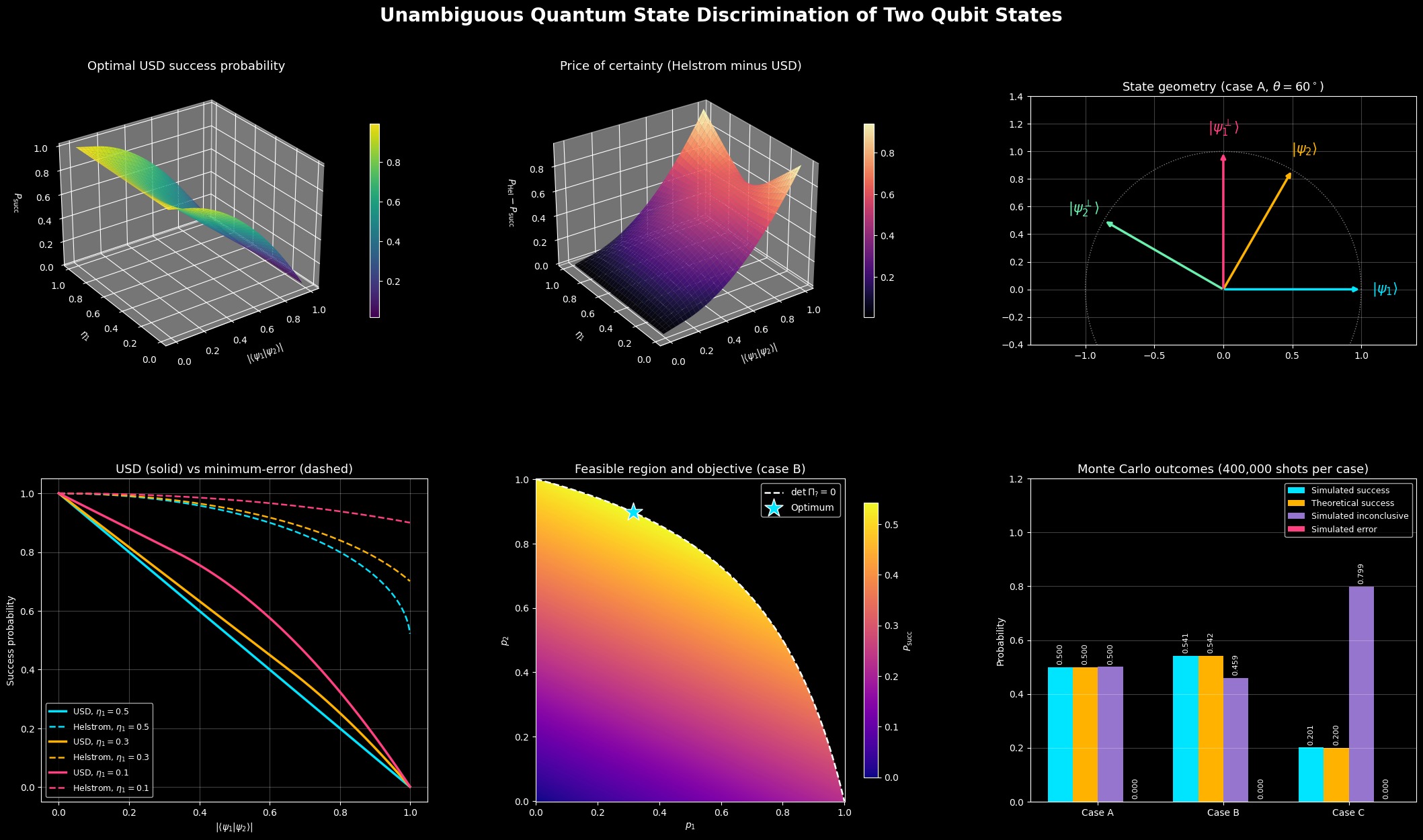
The single figure contains six panels:
- A 3D surface of the optimal success probability over overlap and prior.
- A 3D surface of the gap between the Helstrom bound and USD.
- The geometry of the states and the POVM directions.
- Success-probability curves for several priors.
- The feasible region in the $(p_1,p_2)$ plane.
- The Monte Carlo statistics for the three cases.
The vectorized design (grid evaluation with broadcasting, trace and determinant instead of eigendecomposition, and mask-based sampling) keeps the whole script fast enough to run in a few seconds.
Execution Results
======================================================================================================================
Unambiguous Quantum State Discrimination: theory vs brute force vs Monte Carlo
======================================================================================================================
Case   theta   eta1     |s|       p1       p2    Theory   BruteF.   MC succ  MC error  MC inconc.  Helstrom    min eig
----------------------------------------------------------------------------------------------------------------------
A       60.0   0.50  0.5000   0.6667   0.6667    0.5000    0.5000    0.4996    0.0000      0.5004    0.9330  -4.16e-17
B       60.0   0.30  0.5000   0.3150   0.8969    0.5417    0.5417    0.5413    0.0000      0.4587    0.9444   5.20e-17
C       30.0   0.20  0.8660   0.0000   1.0000    0.2000    0.2000    0.2006    0.0000      0.7994    0.8606   0.00e+00
======================================================================================================================
Shots per case: 400,000
Detailed Discussion of the Results
The success-probability surface
The first 3D panel shows $P_{\mathrm{succ}}$ as a function of the overlap $|s|$ and the prior $\eta_1$. Along the edge $|s|=0$ the surface sits at height $1$, because orthogonal states can be distinguished perfectly. As the overlap grows, the height falls toward $0$ along the edge $|s|\to 1$, where the two states become physically identical. The surface is highest along the central ridge $\eta_1 = 0.5$ at small overlap and bends differently near the edges $\eta_1\to 0$ and $\eta_1 \to 1$. There, the more probable state dominates and the Regime II formula $\max(\eta_1,\eta_2)(1-|s|^2)$ takes over. The kink between the two regimes is where the optimal strategy changes qualitatively.
The price of certainty
The second surface plots $P_{\mathrm{Hel}} - P_{\mathrm{succ}}$. It vanishes at $|s|=0$, since both strategies are perfect for orthogonal states. It also shrinks again near $|s|\to1$, where neither strategy can do much. The largest gap appears at intermediate overlaps and balanced priors. For case A, the theory gives $P_{\mathrm{Hel}}\approx 0.933$ against $P_{\mathrm{succ}}=0.5$. The Helstrom measurement always answers and is right about 93% of the time, whereas the unambiguous measurement answers only half the time but is never wrong.
The geometry panel
The geometry panel shows why the measurement works. The vector $|\psi_2^{\perp}\rangle$ is perpendicular to $|\psi_2\rangle$, so the projector onto it can never fire when the state is $\psi_2$. A click therefore proves the state was $\psi_1$. The same argument applies to $|\psi_1^{\perp}\rangle$ and $\psi_2$. The price is that these two directions are not orthogonal to each other, so they cannot be combined into a complete measurement. The leftover element $\Pi_?$ must absorb the remainder, and that is where the inconclusive outcomes come from.
The curves
The solid curves are the USD optimum and the dashed curves are the Helstrom bound for the same priors. Each dashed curve lies above its solid partner. For $\eta_1 = 0.5$ the solid curve is the straight line $1-|s|$. For biased priors the solid curves follow the Regime I line at first and then switch to the downward parabola $\max(\eta_1,\eta_2)(1-|s|^2)$ after the threshold overlap. The curve is continuous at the threshold, and its slope is continuous there as well, which makes the transition smooth.
The feasible region
The heatmap shows the objective over the feasible region for case B. The white dashed curve is the boundary $\det\Pi_?=0$, and the region below it is feasible. Because the objective is linear, its maximum must lie on this boundary, and the star marks the optimum, with $p_1\approx0.315$ and $p_2\approx 0.897$. The solution gives a larger weight to the less probable state’s identifier, which is a counterintuitive but correct feature of USD with unequal priors: a state that is rarely prepared needs a more aggressive unambiguous test to extract its share of the success probability.
The Monte Carlo statistics
The bar chart compares simulated and theoretical success probabilities for the three cases: $0.5$, about $0.5417$, and $0.2$. The simulated bars agree with the theoretical bars to within statistical fluctuations of order $1/\sqrt{N}$. The most important bar is the pink one. The simulated error rate is exactly zero in all three cases, because the forbidden outcomes have probability zero by construction. The rest of the probability is the inconclusive fraction, so the three bars for each case, success, inconclusive and error, add up to one.
Case C illustrates Regime II. With a small angle and a strongly biased prior, the optimal strategy abandons any attempt to identify the rare state. The measurement only tries to confirm the likely state, with $p_1=0$ and $p_2=1$ in the notation above, and it succeeds with probability $0.8\times(1-0.75)=0.2$. This is a good reminder that the “best” unambiguous measurement is not always symmetric.
Conclusion
Unambiguous state discrimination turns a fundamental quantum limitation into a clean optimization problem. By trading some certainty about whether we get an answer for absolute certainty about what the answer is, we obtain the closed-form optimum
$$
P_{\mathrm{succ}} = 1 - 2\sqrt{\eta_1\eta_2},|\langle\psi_1|\psi_2\rangle|
$$
in the balanced regime, and the simpler $\max(\eta_1,\eta_2)(1-|s|^2)$ in the strongly biased regime. Brute-force search over the feasible region and a Monte Carlo simulation of the explicit POVM both confirm the analysis, and the 3D landscapes show how the optimum depends on both the overlap and the priors. The same framework extends to more than two states, to mixed states, and to discrimination under noise, where the optimization is usually solved numerically with semidefinite programming.