Risk-Optimized Degradation Planning with Python
A satellite lives or dies by its power budget. The solar array is the only source of electricity for the entire mission, yet it is under constant attack from trapped radiation, solar particle events, thermal cycling, and ultraviolet exposure. Every year in orbit, the array delivers a little less power than the year before.
The naive engineering answer is to size the array for the average degradation. That design misses its end-of-life requirement roughly half of the time. The opposite answer is to add a huge safety margin, which costs launch mass, and mass is money. In this article we treat the problem as a chance-constrained optimization and solve it with Monte Carlo simulation in Python.
1. The Problem
We design a solar array for a satellite in a harsh radiation environment (think of a medium-altitude orbit). The mission requirements are:
- Mission life: $T = 15$ years
- Required end-of-life (EOL) power: $P_{\mathrm{req}} = 6000\ \mathrm{W}$
- The probability of falling short of $P_{\mathrm{req}}$ at EOL must not exceed $\alpha = 5%$
We have two design variables:
- $t$: the equivalent shield (coverglass) thickness in mm. A thicker shield blocks more radiation, but it is heavy.
- $A$: the array area in $\mathrm{m}^2$. A larger array produces more power, but it is also heavy.
The objective is to minimize the array mass:
$$
\min_{t,,A}; M(t,A) = A,\bigl(m_0 + \rho,t\bigr)
$$
$$
\text{subject to}\quad \Pr\bigl[,P_{\mathrm{EOL}}(t,A,\omega) \ge P_{\mathrm{req}},\bigr] \ge 1-\alpha
$$
Here $m_0 = 4.2\ \mathrm{kg/m^2}$ is the areal mass of the bare array, $\rho = 2.6\ \mathrm{kg/m^2/mm}$ is the areal mass added per millimeter of shield, and $\omega$ denotes one random scenario.
2. The Degradation Model
The power at end of life is
$$
P_{\mathrm{EOL}} = A, p_{\mathrm{BOL}},\bigl(1 - L_{\mathrm{rad}}\bigr)\bigl(1 - k,T\bigr)
$$
where $p_{\mathrm{BOL}} = S_0,\eta,f_{\mathrm{pack}},f_{\cos},f_{\mathrm{temp}} \approx 306.6\ \mathrm{W/m^2}$ is the beginning-of-life power density.
The radiation loss follows the well-known semi-empirical logarithmic law:
$$
L_{\mathrm{rad}} = C,\log_{10}!\left(1 + \frac{\Phi_{\mathrm{eff}}}{\Phi_x}\right)
$$
The effective fluence behind the shield is attenuated exponentially with thickness. It has two components, a continuous background and the sum of discrete solar particle events (SPEs):
$$
\Phi_{\mathrm{eff}} = \Phi_{\mathrm{bg}},e^{-t/\lambda_{\mathrm{bg}}} + \Phi_{\mathrm{spe}},e^{-t/\lambda_{\mathrm{spe}}}
$$
$$
\Phi_{\mathrm{bg}} = r_{\mathrm{bg}},T, \qquad \Phi_{\mathrm{spe}} = \sum_{j=1}^{N} \phi_j, \qquad N \sim \mathrm{Poisson}(\lambda_{\mathrm{ev}} T)
$$
The random ingredients are:
| Quantity | Distribution |
|---|---|
| Background fluence rate $r_{\mathrm{bg}}$ | Log-normal, median $4\times10^{14}$, $\sigma = 0.30$ |
| SPE fluence per event $\phi_j$ | Log-normal, median $8\times10^{13}$, $\sigma = 1.5$ |
| Number of SPEs $N$ | Poisson, 1 event per year |
| Damage coefficient $C$ | Normal, mean 0.18, std 0.02 |
| Thermal/UV loss rate $k$ | Normal, mean 0.4 %/year, std 0.12 %/year |
3. A Fast Solution Strategy
A brute-force approach would simulate every design pair $(t, A)$ separately. The chance constraint has a much better structure. For a fixed thickness $t$, define the EOL power per unit area $u(t,\omega) = P_{\mathrm{EOL}}/A$. The shortfall event is $A,u < P_{\mathrm{req}}$, and therefore
$$
\Pr\bigl[A,u(t,\omega) \ge P_{\mathrm{req}}\bigr] \ge 1-\alpha
;\Longleftrightarrow;
A \ge A_{\mathrm{req}}(t) = \frac{P_{\mathrm{req}}}{Q_{\alpha}\bigl[u(t,\cdot)\bigr]}
$$
where $Q_\alpha$ is the $\alpha$-quantile of the scenario distribution. The two-dimensional stochastic problem collapses into a one-dimensional deterministic problem:
$$
\min_{t}; M(t) = A_{\mathrm{req}}(t),\bigl(m_0 + \rho,t\bigr)
$$
The full risk map over $(t, A)$ is also cheap. After sorting the scenarios once per thickness, the shortfall probability for any area is a single binary search. All 20,000 scenarios share the same random numbers across every design (common random numbers), which keeps the risk surface smooth and the comparison between designs fair. Everything is vectorized with NumPy, with no Python loop over scenarios.
4. The Complete Source Code
1 | import time |
5. Code Walkthrough
5.1 Parameters
The first block collects every physical and economic assumption in one place. UNIT_POWER_BOL multiplies the solar constant by the cell efficiency, the packing factor, the average cosine loss, and a temperature derating factor, giving about 306.6 W per square meter at beginning of life. M_BASE and RHO_GLASS define the mass model $M = A(m_0 + \rho t)$. The remaining constants describe the radiation environment and the uncertainty of each ingredient.
5.2 Scenario Generation
Each of the 20,000 scenarios carries its own background fluence rate, damage coefficient $C$, and thermal/UV loss rate $k$. Solar particle events need more care because the number of events varies from scenario to scenario. We draw a Poisson count per scenario, then generate a padded matrix of event magnitudes and event times with MAX_EV columns. A boolean mask, EV_MASK, zeroes out the unused columns. Summing along the event axis gives the total SPE fluence per scenario, PHI_SPE_EOL. The event times are kept because we need them later for the power history.
The clipping of $C$ and $k$ keeps the sampled values physically meaningful, since a negative degradation rate has no meaning.
5.3 The Vectorized Core
eol_unit_power is the heart of the model. Given a whole vector of shield thicknesses, it returns a matrix of shape (thickness, scenario). Broadcasting handles the exponential attenuation, the logarithmic radiation law, and the linear thermal/UV loss in a single expression. No Python loop touches the scenarios, so evaluating all 121 thicknesses against 20,000 scenarios takes a fraction of a second.
5.4 Quantile Reduction
The line U_Q = np.quantile(U, ALPHA, axis=1) returns, for every thickness, the power density that 95% of the scenarios exceed. Dividing $P_{\mathrm{req}}$ by it gives the smallest area that satisfies the chance constraint, exactly as derived in Section 3. Multiplying by the areal mass gives the mass curve, and argmin picks the optimal thickness.
5.5 The Risk Map
To draw the full 3D risk surface we still need the shortfall probability for arbitrary $(t, A)$ pairs. Each row of U is sorted once, after which np.searchsorted counts how many scenarios fall below the threshold $P_{\mathrm{req}}/A$ for all 61 areas simultaneously. The loop runs only over the 121 thicknesses, never over scenarios or areas.
5.6 The Price of Confidence
The same quantile trick is repeated for 50 different confidence levels between 50% and 99% with a single call to np.quantile using a vector of probabilities. This yields the minimum achievable mass as a function of the required confidence, which is the practical trade-off a program manager cares about.
5.7 Time History
power_timeseries replays the first 4,000 scenarios through time. At every time step, only the solar particle events that have already occurred contribute to the fluence, while the background fluence grows linearly. The final time step reproduces the EOL values used in the optimization, so the fan chart is consistent with the optimizer.
5.8 Visualization
All six panels are drawn into one figure. The two 3D panels show the risk surface and the mass surface, the latter with infeasible designs painted gray so that the feasible region and the optimum stand out at a glance.
6. Execution Results
========================================================================
 Solar array degradation risk optimisation (chance-constrained design)
========================================================================
 Mission life               : 15 years
 Required EOL power         : 6000 W
 Required confidence        : 95.0 %
 Monte Carlo scenarios      : 20,000
 Design points evaluated    : 121 x 61 = 7,381
 Computation time           : 0.29 s
------------------------------------------------------------------------
 Optimal design
   Shield thickness         : 0.575 mm
   Array area               : 23.01 m^2
   Array mass               : 131.0 kg
   Shortfall probability    : 5.00 %
------------------------------------------------------------------------
 Nominal (median-sized) design at the same thickness
   Array area               : 21.96 m^2
   Array mass               : 125.0 kg
   Shortfall probability    : 50.00 %
------------------------------------------------------------------------
   t [mm]   A_req [m^2]   Mass [kg]   vs optimum [%]
    0.100         35.70       159.2            21.50
    0.200         31.41       148.3            13.14
    0.300         28.18       140.3             7.10
    0.400         25.75       134.9             2.96
    0.575         23.01       131.0             0.00
    0.600         22.75       131.1             0.02
    0.700         22.07       132.9             1.39
========================================================================
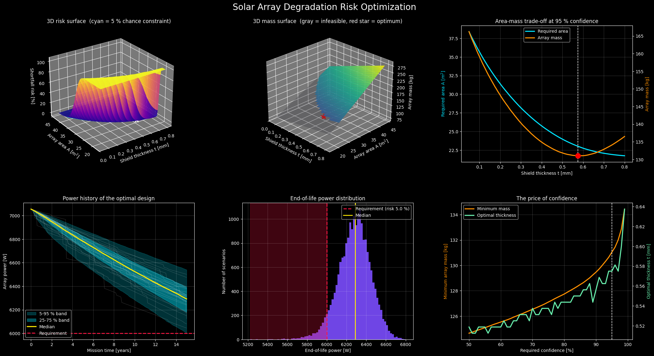
7. Interpreting the Results
The optimal design. With the random seed used here, the optimizer selects a shield thickness of about 0.575 mm and an array area of about 23.0 $\mathrm{m}^2$, for a total array mass of about 131 kg. The Monte Carlo estimate of the shortfall probability is 5.00%, matching the chance constraint with no wasted margin.
The nominal design is a trap. Sizing the array with the median degradation at the same thickness needs only about 22.0 $\mathrm{m}^2$ and 125 kg. That is 6 kg lighter, but it fails to deliver 6000 W in half of all scenarios. The console report shows this clearly: a shortfall probability of 50%.
The 3D risk surface (top left). The surface is close to a cliff. For a given thickness there is a narrow band of areas over which the shortfall probability climbs from nearly 0% to nearly 100%, because the scenario spread is small compared with the design range. The cyan curve marks the 5% level, and every design on or beyond it is acceptable. The optimum lies on that curve, which is exactly what a chance-constrained optimum should do.
The 3D mass surface (top center). The mass grows almost linearly with area, while the effect of thickness is more subtle. The gray region marks infeasible designs. The red star sits on the boundary of the feasible region, at the lowest mass point on it.
The trade-off curve (top right). The required area decreases steadily as the shield gets thicker, because radiation damage shrinks. The mass, however, has a minimum. Thin shields force a large array; thick shields add glass mass faster than they save array mass. At 0.10 mm the array is about 21.5% heavier than the optimum, and at 0.30 mm it is still about 7.1% heavier. The curve is quite flat near the optimum, so a thickness between 0.5 and 0.7 mm costs at most about 1.4% extra mass. Engineers can pick a practical thickness without losing much.
The fan chart (bottom left). The median power falls from about 7050 W at launch to roughly 6300 W after 15 years. The lower edge of the 5-95% band touches the 6000 W requirement line at the end of the mission, which is precisely what a 95% confidence design should look like. The thin white lines are individual scenarios; sudden downward steps are solar particle events.
The EOL distribution (bottom center). The histogram has a longer tail toward low power. Heavy-tailed solar particle events produce rare but severe losses, and the red-shaded region to the left of the requirement contains exactly 5% of the scenarios.
The price of confidence (bottom right). Raising the required confidence from 50% to 99% raises the minimum mass from about 125 kg to about 134 kg, and the curve steepens sharply near the high end. The last few percentage points of reliability are the most expensive ones. Meanwhile, the optimal thickness creeps upward with the required confidence, because a thicker shield suppresses the heavy tail of the fluence distribution.
8. Conclusion
We turned a vague engineering worry into a precise optimization problem: minimize array mass subject to a probabilistic end-of-life power requirement. The key mathematical step was the quantile reduction
$$
A_{\mathrm{req}}(t) = \frac{P_{\mathrm{req}}}{Q_{\alpha}\bigl[u(t,\cdot)\bigr]}
$$
which converts a stochastic two-variable problem into a fast one-dimensional search, and vectorized NumPy evaluates the whole design space in a fraction of a second.
The results deliver three lessons. First, designing for the average is a coin flip. Second, the mass-optimal shield is neither the thinnest nor the thickest, and the optimum is broad enough to leave room for practical engineering judgment. Third, the last few percent of confidence are expensive, so the confidence level itself should be a deliberate management decision.
The same framework extends naturally to other risk drivers: eclipse thermal cycling in different orbits, cell-technology selection, in-orbit annealing, or a multi-objective formulation with launch cost. Only the scenario generator and the mass model need to change.