The Water-Gas Shift Equilibrium
Why Minimizing Gibbs Free Energy Matters
Chemical systems don’t settle into equilibrium by “reacting until reactants run out.” They settle where the total Gibbs free energy of the system is at its minimum at fixed temperature $T$ and pressure $P$. This is one of the most elegant ideas in thermodynamics: instead of solving equilibrium constant equations one reaction at a time, you can treat the whole problem as a constrained optimization problem.
For a mixture of $N$ species, the total Gibbs free energy is:
$$
G(n_1, n_2, \dots, n_N) = \sum_{i=1}^{N} n_i \left[ \mu_i^{\circ}(T) + RT \ln\left(\frac{y_i P}{P^{\circ}}\right) \right]
$$
where:
- $n_i$ = moles of species $i$
- $y_i = n_i / \sum_j n_j$ = mole fraction
- $\mu_i^{\circ}(T)$ = standard chemical potential of species $i$ at temperature $T$
- $R$ = universal gas constant
- $P^{\circ}$ = reference pressure (1 atm)
The equilibrium composition is the set of $n_i$ that minimizes $G$, subject to atomic mass balance constraints:
$$
\sum_{i=1}^{N} a_{ki} , n_i = b_k \quad \text{for each atom } k
$$
where $a_{ki}$ is the number of atoms of element $k$ in species $i$, and $b_k$ is the total amount of element $k$ available from the feed. This formulation (the “direct minimization” method, originally due to White, Johnson & Dantzig) avoids ever writing down an equilibrium constant — the physics falls out entirely from the shape of $G$.
The Example: Water-Gas Shift Reaction
We’ll use a classic industrial reaction:
$$
\text{CO} + \text{H}_2\text{O} ;\rightleftharpoons; \text{CO}_2 + \text{H}_2
$$
This is a single-degree-of-freedom system: 4 species (CO, H₂O, CO₂, H₂), 3 atoms (C, H, O), so there’s exactly one independent reaction extent $\xi$. Starting from 1 mol CO + 1 mol H₂O, we can write:
$$
n_{CO} = 1-\xi,\quad n_{H_2O} = 1-\xi,\quad n_{CO_2} = \xi,\quad n_{H_2} = \xi
$$
We’ll solve the general $n$-dimensional problem with scipy.optimize.minimize (SLSQP), then also verify it against the simple 1-D $\xi$ picture, scan over temperature, and finally map out the equilibrium H₂ mole fraction as a 3D surface over $(T, P)$.
Full Source Code
1 | # ============================================================ |
Detailed Code Walkthrough
Section 1 — Thermodynamic data. We store enthalpy of formation ($\Delta H_f^\circ$) and standard entropy ($S^\circ$) for each of the 4 species, and approximate the temperature-dependent chemical potential as $\mu_i^\circ(T) \approx \Delta H_{f,i}^\circ - T S_i^\circ$. This ignores heat-capacity ($C_p$) corrections, which is a standard simplification for a first-pass teaching example — the qualitative equilibrium behavior it produces is realistic.
The matrix A encodes how many atoms of C, H, and O are in each species (columns = CO, H₂O, CO₂, H₂). Multiplying A by the feed vector gives the conserved atom totals b — this is the constraint the optimizer must respect no matter how the mixture rearranges itself.
gibbs_total(n, T, P) implements the free-energy formula directly: it clips n away from zero (to avoid log(0)), computes mole fractions y, and sums $n_i \mu_i$ over all species.
solve_equilibrium(T, P, x0) is the core optimizer call. It builds 3 equality constraints (one per atom) as lambda closures — note the i=i trick, which is required so each lambda captures its own value of i rather than all sharing the last loop value. Bounds keep every $n_i$ strictly positive (no negative moles). SLSQP (Sequential Least Squares Programming) is used because it natively supports both bounds and nonlinear/linear equality constraints — ideal for this kind of problem.
Section 3 cross-checks the general optimizer against the simple 1-D reaction-extent formulation, where $\xi$ alone fully parametrizes the mixture. Scanning $\xi$ from 0 to 1 and plotting $G(\xi)$ should show a single smooth bowl-shaped curve with one minimum — exactly where minimize_scalar lands, and exactly where the SLSQP solution from Section 2 should agree.
Section 4 solves equilibrium repeatedly across a temperature sweep. The key performance trick is warm-starting: each solve’s result becomes the initial guess (x0) for the next temperature, since equilibrium composition changes only slightly between adjacent grid points. This cuts iteration counts dramatically compared to always starting from the same generic guess.
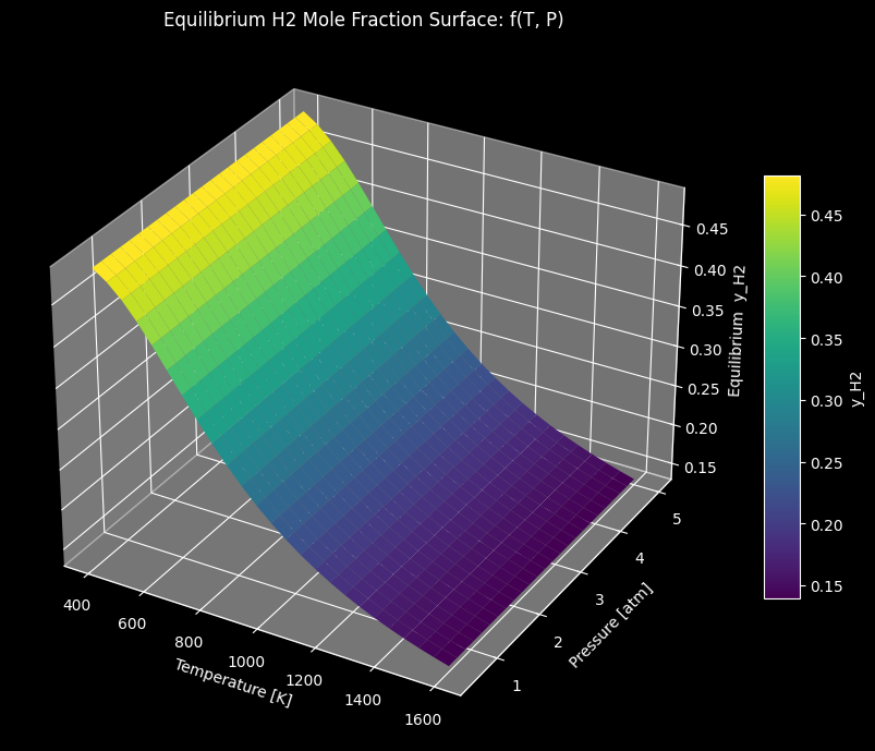
Section 5 extends the same warm-start idea to a full $(T, P)$ grid (25×25 = 625 optimizations), reusing the previous $T$-point’s solution as it sweeps across each pressure row. This keeps the whole grid scan fast even though it’s calling scipy.optimize.minimize hundreds of times.
=== Equilibrium at T=1000K, P=1atm ===
Optimizer success: True | Optimization terminated successfully
  n_CO   = 0.51293 mol   (y_CO = 0.25646)
  n_H2O  = 0.51293 mol   (y_H2O = 0.25646)
  n_CO2  = 0.48707 mol   (y_CO2 = 0.24354)
  n_H2   = 0.48707 mol   (y_H2 = 0.24354)
  G_min = -761468.144 J

All computations finished.
Reading the Graphs
Figure 1 — G vs. reaction extent ξ. This is the most direct visual proof of “free energy minimization” in action: the curve should form a single smooth bowl between $\xi=0$ and $\xi=1$, with the red marker sitting exactly at the bottom. There is no equilibrium constant, no algebra — just literally the lowest point of a curve.
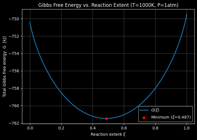
Figure 2 — Composition vs. Temperature. Since $\Delta H_{rxn} = \Delta H_{f,CO_2} + \Delta H_{f,H_2} - \Delta H_{f,CO} - \Delta H_{f,H_2O} \approx -41\text{ kJ/mol}$, the water-gas shift reaction is mildly exothermic. By Le Chatelier’s principle, raising temperature should push the equilibrium back toward the reactants — so you should see $y_{H_2}$ and $y_{CO_2}$ decrease, while $y_{CO}$ and $y_{H_2O}$ increase, as $T$ rises across the scan. This is a genuine physical prediction falling directly out of the optimizer, not hard-coded.
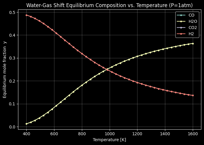
Figure 3 — 3D surface of y_H₂ over (T, P). Look closely at the pressure axis: because this reaction has no change in total gas moles (2 moles of reactants → 2 moles of products), the equilibrium composition is theoretically independent of pressure — the surface should look essentially flat along the $P$ direction while curving strongly along $T$. That’s a subtle but important thermodynamic signature this graph should reveal at a glance: pressure only matters for reactions that change the mole count.
Wrap-Up
What makes this approach powerful is that it generalizes far beyond one reaction: add more species and more atom-balance rows, and the exact same solve_equilibrium function handles arbitrarily complex reacting systems — combustion, gasification, multi-phase equilibria — without ever writing a single equilibrium-constant expression by hand. The physics is entirely encoded in the shape of $G(n)$, and scipy.optimize.minimize does the rest.