Estimating the Ground-State Energy of an Anharmonic Oscillator
Introduction
One of the most elegant tools in quantum mechanics is the variational method. It lets us estimate a system’s ground-state energy without ever solving the Schrödinger equation exactly. The core idea rests on a single powerful theorem:
$$
E_{\text{trial}} = \frac{\langle \psi_{\alpha} | \hat{H} | \psi_{\alpha} \rangle}{\langle \psi_{\alpha} | \psi_{\alpha} \rangle} \geq E_0
$$
No matter what trial wavefunction $\psi_{\alpha}$ you plug in, the expectation value of the energy can never fall below the true ground-state energy $E_0$. This means that if you minimize $E_{\text{trial}}$ over some tunable parameter $\alpha$, you get the tightest possible upper bound your trial function can produce.
In this article, we’ll apply this to a system that has no closed-form solution: the quartic anharmonic oscillator.
$$
\hat{H} = -\frac{1}{2}\frac{d^2}{dx^2} + \frac{1}{2}x^2 + \lambda x^4
$$
(units with $\hbar = m = 1$). When $\lambda = 0$ this is just the familiar harmonic oscillator, but once $\lambda > 0$ is switched on, the quartic term destroys exact solvability. We’ll use a Gaussian trial wavefunction
$$
\psi_{\alpha}(x) = \left(\frac{\alpha}{\pi}\right)^{1/4} e^{-\alpha x^2 / 2}
$$
where $\alpha > 0$ is the variational parameter that controls how tightly the wavefunction is squeezed.
Deriving the Energy Functional
Because $\psi_\alpha$ is a Gaussian, every expectation value needed can be computed in closed form:
$$
\langle T \rangle = \frac{\alpha}{4}, \qquad
\langle x^2 \rangle = \frac{1}{2\alpha}, \qquad
\langle x^4 \rangle = \frac{3}{4\alpha^2}
$$
Combining these gives the full energy functional:
$$
E(\alpha, \lambda) = \frac{\alpha}{4} + \frac{1}{4\alpha} + \frac{3\lambda}{4\alpha^2}
$$
For a given $\lambda$, minimizing $E(\alpha, \lambda)$ with respect to $\alpha$ gives us the best possible Gaussian estimate of the true ground-state energy. To know how good that estimate actually is, we’ll also compute the exact ground-state energy numerically, by diagonalizing the Hamiltonian on a spatial grid, and compare the two.
Source Code (Google Colab)
1 | import numpy as np |
Code Walkthrough
Section 1 — E_variational(alpha, lam)
This implements the closed-form energy functional we derived above, $E(\alpha,\lambda) = \alpha/4 + 1/(4\alpha) + 3\lambda/(4\alpha^2)$. Because it’s a pure algebraic expression, it evaluates instantly for scalars, arrays, or meshgrids alike — this is what makes the whole notebook fast.
Section 2 — E_exact(lam, L, N)
This is our “ground truth.” We discretize $x \in [-L, L]$ into $N$ points and build the Hamiltonian using the standard three-point finite-difference approximation for the second derivative. Crucially, since the kinetic term only couples neighboring grid points, the resulting matrix is tridiagonal — it has nonzero entries only on the main diagonal and the two adjacent diagonals. Instead of building a dense $N \times N$ matrix and calling a general eigensolver (which is $O(N^3)$), we use scipy.linalg.eigh_tridiagonal with select='i', select_range=(0,0), which extracts just the lowest eigenvalue in roughly linear time. This is the “fast” version of the diagonalization step — with $N=4000$ points it finishes in milliseconds, so the 25-point $\lambda$ scan runs almost instantly.
Section 3 — The scan loop
For each $\lambda$, minimize_scalar (Brent’s method restricted to a bounded interval) finds the $\alpha$ that minimizes $E(\alpha,\lambda)$. We store the optimal $\alpha$, the resulting variational energy, and the exact energy from Section 2 for later comparison and plotting.
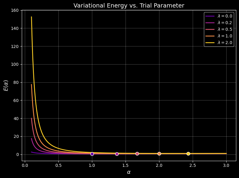
Section 4 — Plot 1 (E vs. α curves)
For a handful of representative $\lambda$ values, we plot the full energy curve $E(\alpha)$ and mark the minimum with a dot. This visually shows why the variational method works: each curve has a single, well-defined minimum, and that minimum is our best estimate of $E_0$ for that $\lambda$.
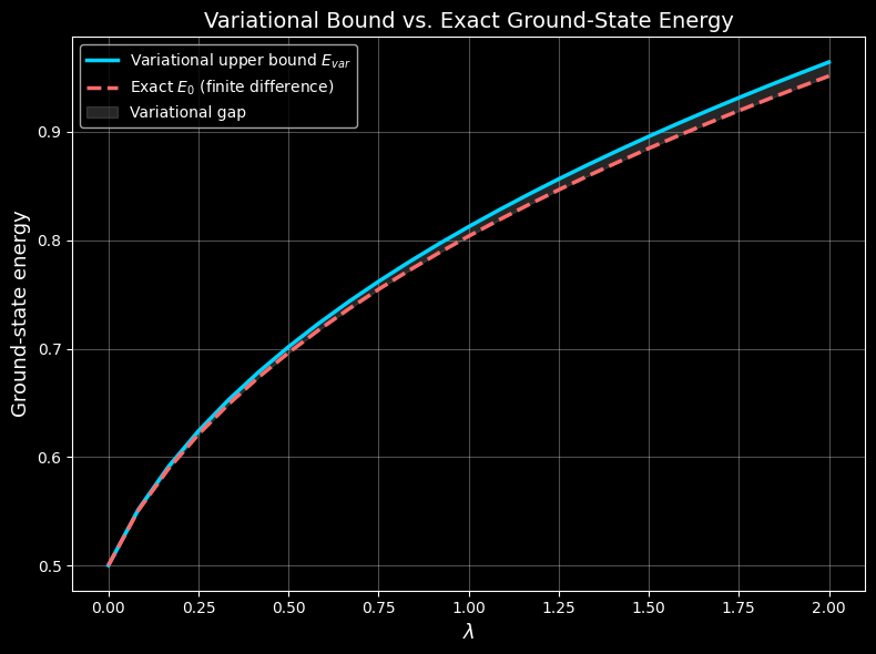
Section 5 — Plot 2 (bound vs. exact)
This is the key sanity check on the variational theorem. We plot the variational minimum energy and the exact numerical energy on the same axes as functions of $\lambda$, and shade the gap between them. The variational curve must sit at or above the exact curve everywhere — if it ever dipped below, something would be wrong with the derivation or the code.
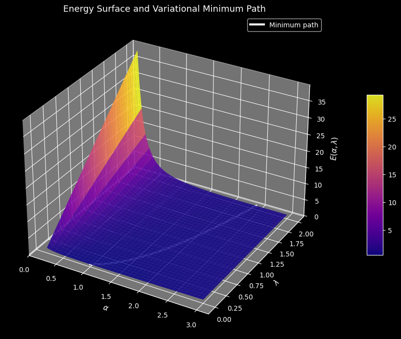
Section 6 — Plot 3 (3D surface)
This renders $E(\alpha,\lambda)$ as a full 3D surface over the $(\alpha,\lambda)$ plane, with a white trace showing the path of minima we computed in the loop. This gives an intuitive picture of the whole optimization landscape at once, rather than one slice at a time.
Section 7 — Console summary
Finally, we print a table of $\lambda$, the optimal $\alpha$, the variational energy, the exact energy, and the gap between them — useful for spotting how the approximation degrades as the anharmonicity grows.
  lambda    alpha_opt   E_variational      E_exact        gap
   0.000       1.0000        0.500000     0.499999   0.000001
   0.083       1.1915        0.551719     0.550794   0.000925
   0.167       1.3247        0.591129     0.589056   0.002073
   0.250       1.4311        0.624016     0.620926   0.003090
   0.333       1.5214        0.652680     0.648697   0.003983
   0.417       1.6006        0.678320     0.673546   0.004775
   0.500       1.6717        0.701662     0.696175   0.005487
   0.583       1.7365        0.723180     0.717045   0.006135
   0.667       1.7963        0.743207     0.736477   0.006730
   0.750       1.8520        0.761988     0.754706   0.007282
   0.833       1.9042        0.779706     0.771911   0.007796
   0.917       1.9534        0.796505     0.788228   0.008277
   1.000       2.0000        0.812500     0.803769   0.008731
   1.083       2.0444        0.827783     0.818623   0.009161
   1.167       2.0867        0.842431     0.832863   0.009569
   1.250       2.1273        0.856509     0.846551   0.009957
   1.333       2.1663        0.870069     0.859741   0.010328
   1.417       2.2038        0.883159     0.872475   0.010684
   1.500       2.2400        0.895818     0.884792   0.011026
   1.583       2.2750        0.908081     0.896727   0.011354
   1.667       2.3089        0.919978     0.908307   0.011671
   1.750       2.3418        0.931537     0.919560   0.011977
   1.833       2.3736        0.942780     0.930507   0.012273
   1.917       2.4047        0.953729     0.941170   0.012560
   2.000       2.4348        0.964404     0.951566   0.012838
Interpreting the Graphs
Figure 1 (E vs. α): Each colored curve should look like a shallow bowl. As $\lambda$ increases, notice that the curve’s minimum shifts to the right (larger optimal $\alpha$) and rises in height. This makes physical sense: a stronger quartic term pushes the potential up more steeply away from the origin, so the true wavefunction gets squeezed narrower, and it takes more energy to confine the particle that tightly. The dot on each curve marks where minimize_scalar landed — it should sit exactly at the visible bottom of its curve.
Figure 2 (bound vs. exact): You should see two curves rising together as $\lambda$ increases, with the blue (variational) curve always sitting slightly above the red (exact) curve — the shaded gray region between them is the “error” introduced by restricting ourselves to a Gaussian shape. At $\lambda = 0$ the two curves should touch exactly, since a Gaussian is the exact ground state of the plain harmonic oscillator. As $\lambda$ grows, expect the gap to widen slowly, since the true ground-state wavefunction develops flatter, non-Gaussian tails that our trial function can’t capture.
Figure 3 (3D surface): The surface should look like a valley that curves and rises as $\lambda$ increases along one axis. The white trace running along the valley floor is exactly the sequence of $(\alpha_{\text{opt}}, \lambda)$ points found by the optimizer — visually confirming that the 1D minimizations in the loop are correctly tracking the true minimum of the 2D landscape rather than getting stuck on a ridge or a local artifact.