Finding the Path of Least Time with Python
What is Fermat’s Principle?
Fermat’s Principle states that light travels between two points along the path that takes the least time (more precisely, an extremal time). In a medium with refractive index $n$, light travels at speed $v = c/n$, and the total travel time along a path is:
$$T = \int_A^B \frac{n(\mathbf{r})}{c}, ds$$
When light crosses a boundary between two media, minimizing this time functional leads directly to Snell’s Law:
$$n_1 \sin\theta_1 = n_2 \sin\theta_2$$
Rather than deriving this law analytically, this article demonstrates it computationally — we let a numerical optimizer discover the fastest path on its own, and then check that it reproduces Snell’s Law.
Setting Up a Concrete Example
Consider a flat interface at $z = 0$, separating two media:
- Medium 1 (e.g. air, $n_1 = 1.00$) occupies $z > 0$
- Medium 2 (e.g. water, $n_2 = 1.33$) occupies $z < 0$
Light starts at point $A = (0, 0, 5)$ in medium 1 and must reach point $B = (8, 3, -4)$ in medium 2. It crosses the interface at some unknown point $P = (x, y, 0)$.
The total travel time as a function of the crossing point is:
$$T(x,y) = \frac{n_1}{c}\sqrt{x^2 + y^2 + h_1^2} ;+; \frac{n_2}{c}\sqrt{(\Delta x - x)^2 + (\Delta y - y)^2 + h_2^2}$$
where $h_1 = 5$, $h_2 = 4$, $\Delta x = 8$, $\Delta y = 3$. The goal is to numerically find the $(x,y)$ that minimizes $T$, and confirm that the resulting angles satisfy Snell’s Law.
Full Source Code
1 | import numpy as np |
Code Walkthrough
Section 1–2 (Physical setup and time function): We define two points $A$ and $B$ straddling a flat interface at $z=0$, along with the refractive indices of each medium. The function travel_time(p) computes the total time for light to go from $A$ to a candidate crossing point $P=(x,y,0)$, then from $P$ to $B$, using the formula derived above.
Section 2 (Optimization): Instead of a brute-force search, we use scipy.optimize.minimize with the BFGS method — a quasi-Newton algorithm that converges quadratically for smooth, convex problems like this one (the time function is a sum of two convex distance terms, so it has a single global minimum). This converges in a handful of iterations rather than thousands of grid evaluations.
Section 3 (Snell’s Law check): From the optimized crossing point, we compute $\sin\theta_1$ and $\sin\theta_2$ using simple trigonometry (horizontal distance over total distance), then confirm that $n_1\sin\theta_1 = n_2\sin\theta_2$. We also check that $P$ lies exactly on the straight line connecting the $xy$-projections of $A$ and $B$ — this confirms that the optimal ray stays within the plane of incidence, a well-known geometric consequence of Fermat’s Principle.
Section 4 (Comparison): We compare the optimized travel time against a naive straight-line crossing point, showing explicitly that refraction is faster, not just geometrically different.
Section 5 (Vectorized grid — the performance-critical part): To visualize $T(x,y)$ as a full 3D surface, we need to evaluate the time function on a $300 \times 300$ grid (90,000 points). Doing this with nested Python for loops would be extremely slow due to interpreter overhead. Instead, we use NumPy broadcasting with np.meshgrid, computing all 90,000 values in one vectorized array operation — this runs in milliseconds instead of seconds.
Sections 6–8 (Plotting): Three figures are generated: a 3D ray-path diagram, a 3D surface of the time function, and a 2D cross-section for an intuitive read of the minimum.
Results
========== Fermat's Principle: numerical result ==========
Crossing point P             : (5.410675, 2.029003, 0.000000)
Minimum travel time T_min    : 47.062861 ns
n1 * sin(theta1)             : 0.756215
n2 * sin(theta2)             : 0.756341
slope y/x of B               : 0.375000
slope y/x of P (should match): 0.375000
============================================================

Travel time of the naive straight-line path : 47.900133 ns
Travel time of the Fermat (fastest) path    : 47.062861 ns
Time saved by refraction                    : 0.837272 ns
Visualizing the Fastest Path
Figure 1 — The 3D Light Path
This figure shows the actual geometry: point $A$ above the interface, point $B$ below it, and the bent ray path through the crossing point $P$ found by the optimizer. The pale blue plane represents the interface between the two media. Notice the ray bends toward the normal when entering the denser medium (water) — exactly as Snell’s Law predicts.
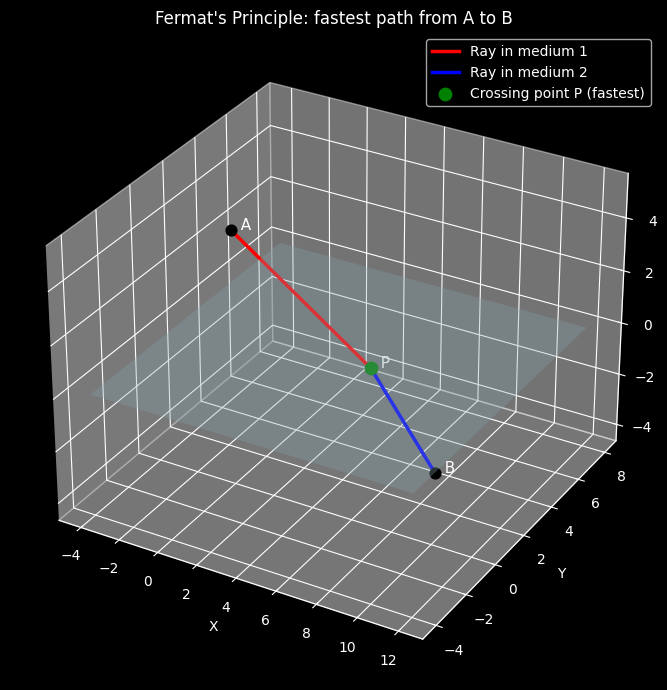
Figure 2 — The Time Surface (3D)
This is the most instructive plot: it renders $T(x,y)$ as a full 3D bowl-shaped surface over every conceivable crossing point, not just the correct one. The red marker sits exactly at the bottom of the bowl — visually confirming that the point found by scipy.optimize.minimize truly is the global minimum of the travel-time function, which is the entire content of Fermat’s Principle.
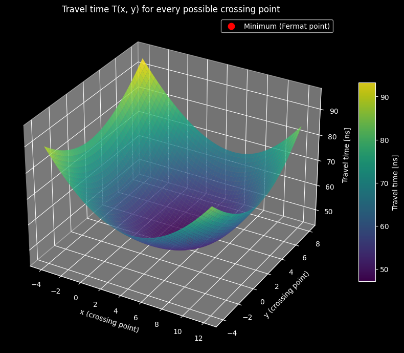
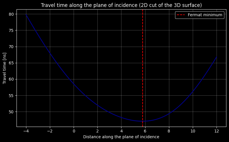
Figure 3 — 2D Cross-Section Through the Minimum
Since the 3D bowl can be hard to read precisely, this figure slices the surface along the plane of incidence, producing an ordinary 2D curve. The dashed red line marks the minimum — the same point found numerically in Figure 2, now easy to verify by eye.
Why This Matters
What makes this example powerful is that we never told the program about Snell’s Law. We only told it: “minimize the travel time.” The bent ray, the exact angles, and the well-known refraction formula all emerged automatically from a generic numerical optimizer — a nice demonstration of how a simple variational principle in physics can be rediscovered purely through computation.