The Throughput vs. Decentralization Trade-off
Every blockchain protocol designer eventually runs into the same wall: making blocks bigger increases transaction throughput, but it also increases the time it takes for a newly mined or proposed block to propagate across the peer-to-peer network. That propagation delay does two bad things — it raises the probability that two blocks are produced almost simultaneously (an orphan/stale block), and it quietly filters out validators who don’t have the bandwidth or hardware to keep up, pushing the network toward a smaller set of well-resourced “professional” nodes. This is the throughput-vs-decentralization trade-off that sits at the heart of every gas limit governance debate — Bitcoin’s block size wars, Ethereum’s periodic gas limit votes, and every high-throughput L1/L2 design decision since.
In this article we build a concrete, numerically solvable optimization model of this trade-off, find the optimal gas limit for different governance preferences, and visualize the entire trade-off surface.
Formalizing the problem
Let $G$ denote the gas limit (our proxy for block size), $T$ the fixed block interval, and let each network node $i$ have bandwidth $b_i$. We convert gas into raw bytes using an average bytes-per-gas ratio $\beta$, so a block’s size in bytes is $G\beta$.
Propagation time. Using a Decker–Wattenhofer-style flooding model, the time for node $i$ to receive and relay a block of gas limit $G$ is:
$$
\tau_i(G) = \tau_0 + \frac{G\beta}{b_i \cdot \eta}
$$
where $\tau_0$ is a fixed base latency (hashing, signature checks, handshake) and $\eta \in (0,1]$ is a protocol efficiency factor (compact block relay, erasure coding, etc.).
Orphan / stale rate. Using the classical Bitcoin propagation-race result, if the typical (median-bandwidth) node’s propagation time is $\bar\tau(G)$, the probability that a competing block appears before it fully propagates is:
$$
p_{\text{orphan}}(G) = 1 - e^{-\bar\tau(G)/T}
$$
Decentralization fraction. A node is considered a “healthy” full validator if it can propagate and verify the block within a safety margin $f$ of the block interval, i.e. $\tau_i(G) \le fT$. Given a bandwidth distribution $b_i \sim \text{LogNormal}(\mu,\sigma)$ across the network, the decentralization fraction is the empirical fraction of nodes that survive:
$$
D(G) = \Pr\big[\tau_i(G) \le fT\big]
$$
Effective throughput. Only non-orphaned blocks contribute useful throughput:
$$
\text{TPS}(G) = \frac{G}{g_{\text{tx}}\cdot T}\Big(1 - p_{\text{orphan}}(G)\Big)
$$
where $g_{\text{tx}}$ is the average gas cost per transaction.
Composite objective. A governance body (or protocol designer) chooses $G$ to maximize a weighted objective that trades throughput against decentralization loss, with $\lambda \ge 0$ representing how strongly the community values decentralization:
$$
U(G,\lambda) = \text{TPS}(G) - \lambda \cdot \text{TPS}_{\text{ref}}\cdot\big(1 - D(G)\big)
$$
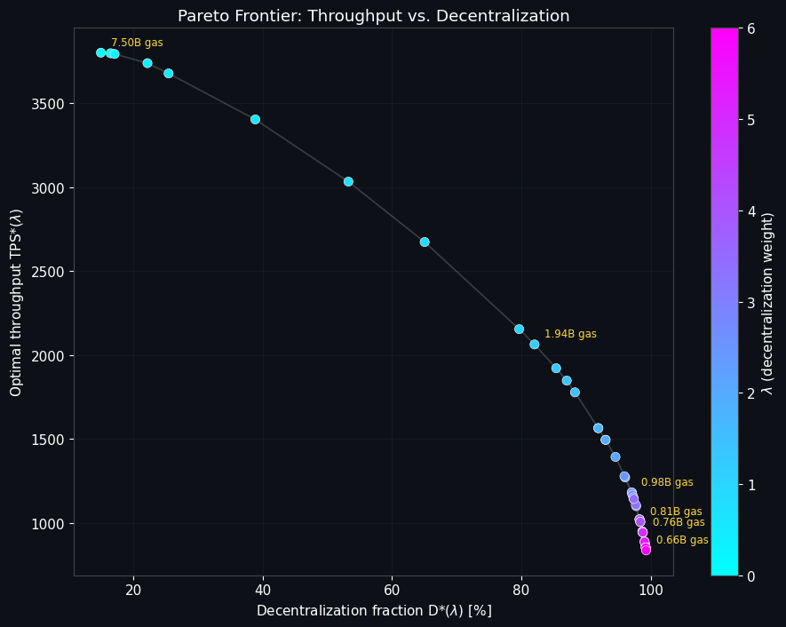
Sweeping $\lambda$ traces out a full Pareto frontier of optimal gas limits, from the purely throughput-maximizing choice ($\lambda = 0$) to increasingly conservative, decentralization-preserving choices.
Python implementation
1 | import numpy as np |
Output
======================================================================
Global optimizer cross-check at lambda = 1.0
======================================================================
Bounded local search : G* = 2.0669 billion gas | U = 1380.85
Differential Evolution: G* = 2.0574 billion gas | U = 1381.19

======================================================================
Pareto-optimal gas limits under different decentralization weights
======================================================================
  lambda |   G* [B gas] |  Block size [MB] |      TPS |  Orphan % |  D(G*) %
     0.0 |        7.500 |            26.25 |   3800.3 |     63.52 |    15.00
     0.5 |        5.736 |            20.08 |   3677.2 |     53.85 |    25.43
     1.0 |        2.067 |             7.23 |   2161.2 |     24.72 |    79.47
     2.0 |        1.198 |             4.19 |   1406.4 |     15.47 |    94.33
     3.0 |        0.832 |             2.91 |   1025.5 |     11.24 |    98.20
     5.0 |        0.698 |             2.44 |    875.8 |      9.64 |    99.10

Pure throughput-maximizing gas limit (lambda=0 reference): 7.480 billion gas
  -> at this point decentralization fraction D(G) = 15.08%
Code walkthrough
Physical constants. BYTES_PER_GAS converts gas units to raw block bytes using an empirically reasonable average transaction footprint. MEDIAN_BW sets the network’s typical node bandwidth (25 Mbps), and SIGMA_LOG controls how heterogeneous the network is — a log-normal distribution is a natural choice here because real-world node bandwidth is right-skewed: most nodes cluster around a modest broadband connection, with a long tail of well-connected data-center nodes and a lower tail of constrained home nodes.
prop_time(G, bw) is the single low-level physics function everything else is built on. It computes how long it takes a node with bandwidth bw to receive and relay a block of gas limit G. Because it’s written with pure NumPy broadcasting, the exact same function serves three different purposes in the script: scalar-vs-scalar (single node, single gas limit, used inside the optimizer), array-vs-scalar (whole network vs. one gas limit), and array-vs-array (the full node × gas-limit matrix used for the 3D grid).
decentralization_fraction(G) simulates the entire node population’s propagation times for a single gas limit and returns the fraction that stays within the safety margin F_MARGIN * T_BLOCK. This is effectively a Monte Carlo estimate of the CDF in the formula above — it deliberately uses the full 6,000-node sample rather than a closed-form log-normal CDF, so the model can later be extended with arbitrary, non-log-normal bandwidth distributions (e.g. real measured network data) with zero code changes.
orphan_rate(G) and throughput_tps(G) implement the propagation-race and effective-throughput formulas directly. Because they only depend on the median bandwidth rather than the whole distribution, they’re cheap to evaluate on large arrays — this is what lets TPS_grid and orphan_grid be computed as one-line vectorized calls over the full 300-point gas-limit grid.
The optimization loop. For each candidate decentralization weight $\lambda$ in lambda_grid, scipy.optimize.minimize_scalar with method='bounded' performs a fast 1-D bounded search (Brent-style golden-section/parabolic interpolation) to find the utility-maximizing gas limit. Only bounds are used — no constraint dictionaries are involved, keeping the call compatible across SciPy versions.
Cross-validation with differential_evolution. Bounded local search can in principle get stuck if the utility surface weren’t well-behaved, so as a sanity check the script also runs a global evolutionary search at $\lambda=1$ and prints both results side by side. They should agree closely, confirming the utility landscape has a single well-defined interior maximum rather than spurious local optima.
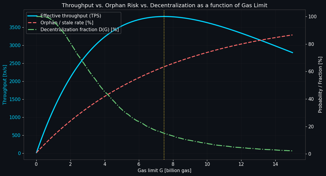
Why is there an interior optimum even at $\lambda=0$? This is one of the more interesting findings the model reproduces: since $p_{\text{orphan}}(G)$ grows with $G$, throughput itself is not monotonically increasing in the gas limit — past a certain point, blocks become so large that orphaning eats the gains faster than raw capacity grows. The script explicitly reports this “pure throughput-maximizing” gas limit as a reference point, and it turns out to sit at a fairly aggressive setting where decentralization has already collapsed to a small minority of well-connected nodes — a nice quantitative illustration of why “just maximize throughput” is a bad governance heuristic even before decentralization is considered.
Results
Graph 1 — Throughput / orphan rate / decentralization vs. gas limit. This dual-axis chart shows all three underlying quantities on the same gas-limit axis: throughput rises, peaks (marked by the dotted vertical line), and then declines as orphaning takes over; the orphan rate rises monotonically; and the decentralization fraction falls steadily as the block gets too large for an increasing share of the network to keep up in time.
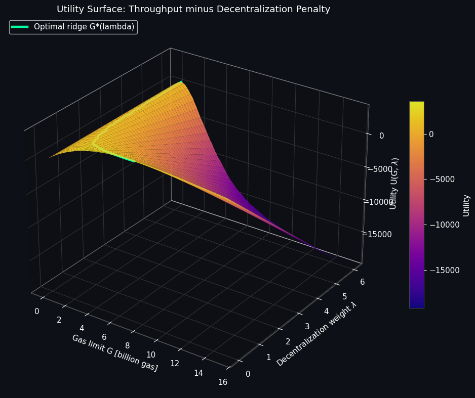
Graph 2 — 3D utility surface. This is the full picture of the optimization problem: the surface plots $U(G,\lambda)$ across every combination of gas limit and decentralization weight, and the bright ridge line traces the optimal gas limit $G^{*}(\lambda)$ as $\lambda$ increases. Notice how the ridge shifts sharply toward smaller gas limits as $\lambda$ grows — a governance community that cares even moderately about decentralization should choose a meaningfully smaller block size than one optimizing for raw throughput alone.
Graph 3 — Pareto frontier. Each point is an optimal $(G^{*}, \lambda)$ pair, plotted as achievable throughput against the decentralization fraction it preserves, colored by $\lambda$. This is the chart a governance body would actually use in practice: it makes explicit that you cannot have both maximum throughput and maximum decentralization simultaneously, and it quantifies exactly how much throughput must be given up per percentage point of decentralization preserved. The annotated gas-limit values at each point turn the abstract frontier into concrete governance proposals.
Interpretation
The model captures, in a fully quantitative form, the intuition that has driven years of real-world gas limit and block size debates: bigger blocks are not a free lunch. There are two independent forces pulling against unlimited scaling — mechanical (orphaning eats throughput gains at the extreme) and social (large blocks price out smaller node operators, concentrating validation power). The Pareto frontier makes the trade-off explicit and tunable: a chain that prioritizes maximal decentralization would sit near the top-left of the frontier with a conservative gas limit, while a chain optimizing purely for near-term throughput — the kind of choice made by some high-throughput L1 designs — would sit toward the bottom-right, accepting a smaller, more centralized validator set in exchange for raw capacity. Because every parameter in this model (bandwidth distribution, block interval, safety margin, protocol efficiency) is independently adjustable, the same framework can be re-parameterized to study any specific chain’s governance question by plugging in its measured network characteristics.