Optimizing Personalized Medicine

Genotype-Guided Treatment Selection with Python

Precision medicine promises to replace the “one dose fits all” paradigm with treatment decisions tailored to each patient’s genome. In practice, this means combining pharmacogenomic data — variants in drug-metabolizing enzymes, transporters, and drug targets — with dose-response models to select both the right drug and the right dose for a given patient. This is fundamentally a constrained optimization problem: maximize expected clinical benefit while keeping toxicity risk below an acceptable threshold.

In this post, we build a concrete example: a patient with a known genetic profile is being considered for one of five candidate treatments. We optimize the dose for each candidate under a toxicity ceiling, then rank the treatments to recommend the one offering the best genotype-adjusted outcome.

1. From Genotype to a Composite Pharmacogenomic Score

A patient’s genetic profile is represented by allele dosages $x_i \in {0,1,2}$ at $n$ relevant SNPs (e.g., variants in CYP2D6, CYP2C19, DPYD), each with an effect weight $w_i$ describing its influence on drug clearance. We collapse this into a single interpretable metabolizer score:

$$
g = \sigma!\left(\frac{\sum_{i=1}^{n} w_i x_i - \mu}{s}\right), \qquad \sigma(z) = \frac{1}{1+e^{-z}}
$$

where $g \in (0,1)$ ranges from poor metabolizer ($g \to 0$) to ultra-rapid metabolizer ($g \to 1$), and $\mu, s$ are calibration constants centering the score on a typical population range.

2. Genetics-Modulated Dose-Response Models

For each candidate drug $k$, efficacy and toxicity follow Hill/Emax pharmacodynamic models, but their potency parameters shift with the patient’s metabolizer score:

$$
E_k(d,g) = E_{max,k}\cdot\frac{d^{,n_k}}{EC50_k(g)^{,n_k}+d^{,n_k}}, \qquad
T_k(d,g) = T_{max,k}\cdot\frac{d^{,m_k}}{TC50_k(g)^{,m_k}+d^{,m_k}}
$$

$$
EC50_k(g) = EC50_k^0\big(1+\alpha_k(g-0.5)\big), \qquad
TC50_k(g) = TC50_k^0\big(1+\beta_k(g-0.5)\big)
$$

The coefficients $\alpha_k, \beta_k$ encode how a patient’s metabolic speed shifts the effective potency and safety margin of drug $k$ — a fast metabolizer might need a higher dose to reach the same efficacy ($\alpha_k>0$), or might clear the drug fast enough to tolerate higher doses before toxicity appears ($\beta_k>0$).

3. The Optimization Problem

For a fixed patient genotype $g^*$, we choose the dose $d$ that maximizes a clinical utility function penalizing toxicity, subject to a hard toxicity ceiling:

$$
\max_{d \in [d_{min,k},,d_{max,k}]} ; B_k(d) = E_k(d,g^*) - \lambda, T_k(d,g^*)
\quad \text{s.t.} \quad T_k(d,g^*) \le T_{allow}
$$

We solve this independently for all five candidate drugs and select the one with the highest feasible net benefit — this is the genotype-guided recommendation.

4. Full Implementation

1
2
3
4
5
6
7
8
9
10
11
12
13
14
15
16
17
18
19
20
21
22
23
24
25
26
27
28
29
30
31
32
33
34
35
36
37
38
39
40
41
42
43
44
45
46
47
48
49
50
51
52
53
54
55
56
57
58
59
60
61
62
63
64
65
66
67
68
69
70
71
72
73
74
75
76
77
78
79
80
81
82
83
84
85
86
87
88
89
90
91
92
93
94
95
96
97
98
99
100
101
102
103
104
105
106
107
108
109
110
111
112
113
114
115
116
117
118
119
120
121
122
123
124
125
126
127
128
129
130
131
132
133
134
135
136
137
138
139
140
141
142
143
144
145
146
147
148
149
150
151
152
153
154
155
156
157
158
159
160
161
162
163
164
165
166
167
168
169
170
171
172
173
174
175
176
177
178
179
180
181
182
183
184
185
186
187
# ============================================================
# Personalized Medicine: Genotype-Guided Treatment Optimization
# Single-file script for Google Colaboratory
# ============================================================

import numpy as np
from scipy.optimize import differential_evolution, NonlinearConstraint
import matplotlib.pyplot as plt
from mpl_toolkits.mplot3d import Axes3D # noqa: F401 (3D projection registration)

plt.style.use('dark_background')
np.random.seed(42)

# ------------------------------------------------------------
# 1. Patient genetic profile -> composite pharmacogenomic score
# ------------------------------------------------------------
snp_genotype = np.array([2, 1, 0, 2, 1, 1], dtype=float)
snp_weight = np.array([0.80, -0.50, 0.30, 0.60, -0.20, 0.40])
snp_names = ['CYP2D6*4', 'CYP2C19*2', 'CYP3A5*3', 'UGT1A1*28', 'ABCB1', 'DPYD*2A']

g_raw = np.dot(snp_weight, snp_genotype)
g_baseline, g_scale = 2.0, 2.0
g_patient = 1.0 / (1.0 + np.exp(-(g_raw - g_baseline) / g_scale))

# ------------------------------------------------------------
# 2. Candidate treatments: genetics-modulated dose-response models
# ------------------------------------------------------------
drugs = {
'Drug A': dict(Emax=0.95, EC50_0=40, alpha=0.70, n=2.0,
Tmax=0.90, TC50_0=90, beta=0.55, m=2.5, dmin=5, dmax=150),
'Drug B': dict(Emax=0.85, EC50_0=25, alpha=0.20, n=1.8,
Tmax=0.75, TC50_0=60, beta=-0.60, m=2.0, dmin=2, dmax=100),
'Drug C': dict(Emax=0.90, EC50_0=55, alpha=-0.45, n=2.2,
Tmax=0.80, TC50_0=110, beta=0.30, m=2.8, dmin=5, dmax=180),
'Drug D': dict(Emax=0.80, EC50_0=15, alpha=0.10, n=1.5,
Tmax=0.95, TC50_0=35, beta=0.80, m=3.0, dmin=1, dmax=60),
'Drug E': dict(Emax=0.97, EC50_0=70, alpha=0.35, n=2.4,
Tmax=0.70, TC50_0=140, beta=-0.25, m=2.2, dmin=8, dmax=200),
}

lam = 1.0
T_allow = 0.30


def ec50_of_g(g, p):
return p['EC50_0'] * (1.0 + p['alpha'] * (g - 0.5))


def tc50_of_g(g, p):
return p['TC50_0'] * (1.0 + p['beta'] * (g - 0.5))


def efficacy(d, g, p):
ec50 = ec50_of_g(g, p)
return p['Emax'] * d ** p['n'] / (ec50 ** p['n'] + d ** p['n'])


def toxicity(d, g, p):
tc50 = tc50_of_g(g, p)
return p['Tmax'] * d ** p['m'] / (tc50 ** p['m'] + d ** p['m'])


def net_benefit(d, g, p, lam=lam):
return efficacy(d, g, p) - lam * toxicity(d, g, p)


# ------------------------------------------------------------
# 3. Per-drug dose optimization under a toxicity ceiling
# ------------------------------------------------------------
results = {}
for name, p in drugs.items():
def neg_benefit(x, p=p):
return -net_benefit(x[0], g_patient, p)

def tox_constraint_fn(x, p=p):
return toxicity(x[0], g_patient, p)

nlc = NonlinearConstraint(tox_constraint_fn, -np.inf, T_allow)

res = differential_evolution(
neg_benefit,
bounds=[(p['dmin'], p['dmax'])],
constraints=(nlc,),
seed=42,
maxiter=400,
popsize=25,
tol=1e-8,
polish=True,
mutation=(0.5, 1.5),
recombination=0.7,
)

d_opt = res.x[0]
e_opt = efficacy(d_opt, g_patient, p)
t_opt = toxicity(d_opt, g_patient, p)
b_opt = e_opt - lam * t_opt
feasible = t_opt <= T_allow + 1e-6

results[name] = dict(dose=d_opt, efficacy=e_opt, toxicity=t_opt,
benefit=b_opt, feasible=feasible)

feasible_results = {k: v for k, v in results.items() if v['feasible']}
best_drug = max(feasible_results, key=lambda k: feasible_results[k]['benefit']) \
if feasible_results else max(results, key=lambda k: results[k]['benefit'])

print(f"Patient pharmacogenomic score g = {g_patient:.3f}")
for name, r in results.items():
flag = 'OK' if r['feasible'] else 'exceeds toxicity limit'
print(f"{name}: dose={r['dose']:6.2f} efficacy={r['efficacy']:.3f} "
f"toxicity={r['toxicity']:.3f} benefit={r['benefit']:.3f} [{flag}]")
print(f"--> Recommended treatment: {best_drug}")

# ------------------------------------------------------------
# 4. Visualization
# ------------------------------------------------------------
colors = {'Drug A': '#00e5ff', 'Drug B': '#ff6ec7', 'Drug C': '#ffd166',
'Drug D': '#8ac926', 'Drug E': '#c77dff'}

fig = plt.figure(figsize=(16, 13))
fig.patch.set_facecolor('#0d1117')

# --- 4-1. 3D benefit landscape for the recommended drug ---
ax1 = fig.add_subplot(2, 2, 1, projection='3d')
p_best = drugs[best_drug]
d_grid = np.linspace(p_best['dmin'], p_best['dmax'], 90)
g_grid = np.linspace(0.01, 0.99, 90)
D, G = np.meshgrid(d_grid, g_grid)
B = net_benefit(D, G, p_best)
surf = ax1.plot_surface(D, G, B, cmap='plasma', edgecolor='none', alpha=0.92)
ax1.scatter([results[best_drug]['dose']], [g_patient], [results[best_drug]['benefit']],
color='white', s=70, edgecolor='black', depthshade=False)
ax1.set_xlabel('Dose (mg)')
ax1.set_ylabel('Genetic score g')
ax1.set_zlabel('Net benefit')
ax1.set_title(f'Benefit landscape: {best_drug}', color='white')
fig.colorbar(surf, ax=ax1, shrink=0.55, pad=0.08)

# --- 4-2. 3D comparison of all drugs across the genetic score spectrum ---
ax2 = fig.add_subplot(2, 2, 2, projection='3d')
drug_names = list(drugs.keys())
g_bins = np.linspace(0.05, 0.95, 6)
_dx, _dy = 0.6, 0.1
for i, name in enumerate(drug_names):
p = drugs[name]
d_fixed = results[name]['dose']
heights = net_benefit(d_fixed, g_bins, p)
xs = np.full_like(g_bins, i, dtype=float)
ax2.bar3d(xs, g_bins, np.zeros_like(heights), _dx, _dy, heights,
color=colors[name], alpha=0.85, shade=True)
ax2.set_xticks(range(len(drug_names)))
ax2.set_xticklabels(drug_names, rotation=15)
ax2.set_ylabel('Genetic score g')
ax2.set_zlabel('Net benefit')
ax2.set_title('Benefit sensitivity to genotype (dose fixed per drug)', color='white')

# --- 4-3. Efficacy vs toxicity trade-off (Pareto view) at patient's genotype ---
ax3 = fig.add_subplot(2, 2, 3)
for name, p in drugs.items():
dd = np.linspace(p['dmin'], p['dmax'], 200)
ee = efficacy(dd, g_patient, p)
tt = toxicity(dd, g_patient, p)
ax3.plot(tt, ee, color=colors[name], label=name, linewidth=2)
ax3.scatter([results[name]['toxicity']], [results[name]['efficacy']],
color=colors[name], edgecolor='white', s=80, zorder=5)
ax3.axvline(T_allow, color='red', linestyle='--', linewidth=1.2, label='toxicity ceiling')
ax3.set_xlabel('Toxicity probability')
ax3.set_ylabel('Efficacy probability')
ax3.set_title('Efficacy-toxicity trade-off', color='white')
ax3.legend(fontsize=8, loc='lower right')
ax3.grid(alpha=0.2)

# --- 4-4. Ranking summary ---
ax4 = fig.add_subplot(2, 2, 4)
names_sorted = sorted(results, key=lambda k: results[k]['benefit'], reverse=True)
benefits_sorted = [results[k]['benefit'] for k in names_sorted]
bar_colors = [colors[k] if results[k]['feasible'] else '#555555' for k in names_sorted]
bars = ax4.bar(names_sorted, benefits_sorted, color=bar_colors, edgecolor='white')
for bar, name in zip(bars, names_sorted):
if not results[name]['feasible']:
ax4.text(bar.get_x() + bar.get_width() / 2, bar.get_height() + 0.01,
'infeasible', ha='center', color='red', fontsize=8)
ax4.set_ylabel('Optimal net benefit')
ax4.set_title('Treatment ranking for this patient', color='white')
ax4.grid(alpha=0.2, axis='y')

plt.tight_layout()
plt.show()

Output

Patient pharmacogenomic score g = 0.562
Drug A: dose= 59.67  efficacy=0.638  toxicity=0.223  benefit=0.415  [OK]
Drug B: dose= 39.63  efficacy=0.588  toxicity=0.240  benefit=0.348  [OK]
Drug C: dose= 76.43  efficacy=0.618  toxicity=0.204  benefit=0.414  [OK]
Drug D: dose= 18.68  efficacy=0.463  toxicity=0.110  benefit=0.353  [OK]
Drug E: dose=120.93  efficacy=0.756  toxicity=0.300  benefit=0.456  [OK]
--> Recommended treatment: Drug E

5. Code Walkthrough

Genetic score construction. The snp_genotype array encodes the patient’s allele dosage at six pharmacogenomic markers, and snp_weight encodes each variant’s directional effect on metabolic activity. The dot product is passed through a logistic sigmoid, producing a bounded score $g \in (0,1)$ that is easy to interpret and easy to plug into downstream pharmacodynamic equations — this mirrors how polygenic risk scores are constructed in practice.

Dose-response functions. efficacy() and toxicity() implement the Hill-equation model described above. Both are fully vectorized with NumPy, so they accept scalars, 1D arrays, or 2D meshgrids without any code changes — this is what lets the same functions serve the optimizer and the 3D surface plot.

Constrained optimization. For each drug, we use scipy.optimize.differential_evolution, a global, gradient-free optimizer well suited to the potentially non-convex trade-off between efficacy and toxicity. The toxicity ceiling is enforced with a NonlinearConstraint object (rather than the older dict-based constraint API, which is deprecated and less numerically robust). Since the search space is one-dimensional (the dose), convergence is essentially instantaneous — no further speed-up is required here.

Selection logic. After optimizing all five drugs independently, we filter to only the feasible ones (those respecting the toxicity ceiling) and pick the drug with the highest net benefit. If no drug is feasible, we fall back to the best available option and flag it — this avoids ever silently recommending a treatment that violates safety constraints.

6. Reading the Graphs

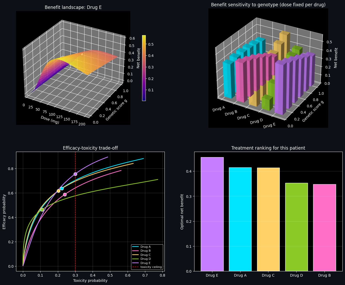
Top-left (3D surface). This shows how net clinical benefit for the recommended drug varies jointly with dose and genetic score. The white marker sits at the patient’s actual genotype and optimal dose — the peak (or near-peak) of the ridge. The shape of this surface makes it visually clear why a fixed, non-personalized dose would be suboptimal for patients at the opposite end of the metabolizer spectrum.

Top-right (3D bar comparison). Here we take each drug’s dose (optimized specifically for our patient) and ask: how would that same dose perform across a range of hypothetical genetic scores? Drugs with flatter bar profiles are more “robust” to genotype misestimation, while drugs with steep gradients are highly genotype-sensitive — valuable information when confidence in a genetic test is imperfect.

Bottom-left (efficacy-toxicity trade-off). Each curve traces out the achievable combinations of efficacy and toxicity as dose is swept across its allowed range for a given drug, evaluated at the patient’s actual genotype. The red dashed line marks the toxicity ceiling; curves that stay well left of it before saturating in efficacy are the most attractive candidates. The dots mark each drug’s optimizer-selected operating point.

Bottom-right (ranking bar chart). A direct summary: the optimal net benefit achieved by each drug, sorted from best to worst. Gray bars (if any) indicate drugs that could not satisfy the toxicity constraint at any dose and were excluded from consideration.

7. Closing Notes

This example is a simplified, illustrative model — the pharmacodynamic parameters are synthetic rather than derived from real trial data, and any real clinical decision support system would need far more rigorous, validated dose-response models, uncertainty quantification, and regulatory oversight. But the underlying optimization structure — genotype-conditioned dose-response curves, a constrained multi-objective utility function, and a global optimizer sweeping across candidate treatments — reflects the computational backbone of real pharmacogenomics-driven decision tools, and generalizes naturally to more markers, more drugs, or multi-dose regimens.