A Fuel-vs-Time Optimization in Python
Geomagnetic storms inflate the upper atmosphere. For satellites flying in low Earth orbit, that means extra drag, faster orbital decay, and — critically for a constellation — satellites drifting out of their assigned slots at different rates depending on their individual ballistic coefficients. Once the storm subsides, ground controllers face a classic operations problem: which satellite should be sent to which slot, and how, so that the total propellant spent and the total time needed to restore the constellation are both kept as low as possible.
This post walks through a concrete example: an 8-satellite constellation in a 700 km circular orbit, hit by a 12-hour geomagnetic storm. We’ll build a decay model, derive the recovery maneuvers (Hohmann transfer + phasing orbit), formulate the satellite-to-slot assignment as a Hungarian-algorithm problem with a tunable fuel/time weight, and visualize everything — including a 3D view of the constellation before and after reconfiguration.
1. Modeling the Problem
1.1 Orbital decay during the storm
Each satellite’s semi-major axis $a_i(t)$ decreases according to a drag-driven decay rate that is amplified during the storm by a Gaussian-shaped intensity pulse $S(t)$:
$$
\frac{da_i}{dt} = -k_i , S(t), \qquad
S(t) = 1 + A_{\text{storm}} \exp!\left(-\frac{(t-t_{\text{peak}})^2}{2\sigma^2}\right)
$$
Here $k_i$ is a satellite-specific decay coefficient (representing small differences in ballistic coefficient between units), $A_{\text{storm}}$ is the drag amplification factor, and $\sigma$ controls the storm’s duration.
As $a_i(t)$ shrinks, the satellite’s mean motion $n_i(t) = \sqrt{\mu/a_i(t)^3}$ increases, so it drifts ahead of its nominal slot. The accumulated phase drift is:
$$
\Delta\theta_i = \int_0^{T_{\text{storm}}} \big(n_i(t) - n_0\big), dt, \qquad n_0 = \sqrt{\mu/a_0^3}
$$
1.2 Recovering altitude: the Hohmann transfer
To return from the decayed altitude $a_f$ to the nominal altitude $a_0$, a two-burn Hohmann transfer is used, with transfer orbit semi-major axis $a_t = (a_f+a_0)/2$:
$$
\Delta v_H = \left|v_{t1}-v_1\right| + \left|v_2-v_{t2}\right|, \qquad
t_H = \pi\sqrt{\frac{a_t^3}{\mu}}
$$
where $v_1=\sqrt{\mu/a_f}$, $v_2=\sqrt{\mu/a_0}$, and $v_{t1},v_{t2}$ are the transfer-orbit speeds at the two burn points. A Hohmann transfer always delivers the satellite to the point diametrically opposite ($\Delta\theta=\pi$) its starting position — this geometric fact turns out to matter a lot for the assignment problem below.
1.3 Correcting phase: the phasing orbit
After the Hohmann transfer, the satellite is at the right altitude but generally at the wrong true anomaly. The remaining phase error $\Delta\phi$ is removed using a phasing orbit: the satellite temporarily shifts to an orbit of period $T_p$ for $n_p$ revolutions, then returns to the target orbit.
$$
T_p = T_0\left(1-\frac{\Delta\phi}{2\pi n_p}\right), \qquad
a_p = \left(\mu\left(\frac{T_p}{2\pi}\right)^2\right)^{1/3}
$$
$$
\Delta v_P = 2\left|v_p - v_{\text{circ}}\right|, \qquad t_P = n_p T_p
$$
Choosing a larger $n_p$ brings $a_p$ closer to $a_0$, lowering $\Delta v_P$ at the cost of more time — exactly the fuel/time trade-off we want to optimize.
1.4 The assignment problem
For every satellite $i$ and every target slot $j$, the total cost is $\Delta v_{ij} = \Delta v_{H,i} + \Delta v_{P,ij}$ and $t_{ij} = t_{H,i} + t_{P,ij}$. Given a weight $\alpha \in [0,1]$, we normalize both matrices to $[0,1]$ and combine them:
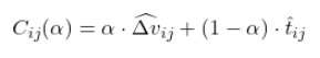
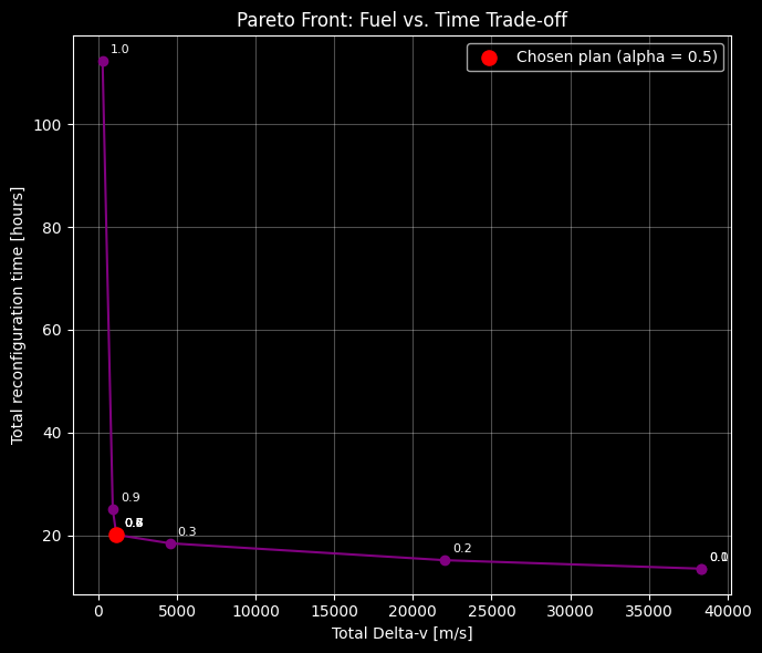
The optimal satellite-to-slot mapping is the permutation $\sigma$ minimizing $\sum_i C_{i,\sigma(i)}(\alpha)$ — solved exactly with the Hungarian algorithm (scipy.optimize.linear_sum_assignment). Sweeping $\alpha$ from 0 to 1 traces out the Pareto front between total fuel and total reconfiguration time.
2. Full Source Code
The whole pipeline is fully vectorized with NumPy (no Python-level loops over time steps or satellite pairs), so it runs essentially instantly even though it covers decay simulation, maneuver design for all 64 satellite-slot pairs across 8 phasing options, and an 11-point Pareto sweep.
1 | import numpy as np |
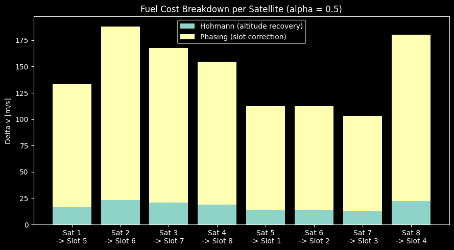
Optimal reconfiguration plan (alpha = 0.5, balanced fuel/time)
============================================================
Satellite 1 -> Slot 5 : dv = 133.46 m/s , time =  2.51 h , phasing loops = 1
Satellite 2 -> Slot 6 : dv = 188.12 m/s , time =  2.52 h , phasing loops = 1
Satellite 3 -> Slot 7 : dv = 167.46 m/s , time =  2.52 h , phasing loops = 1
Satellite 4 -> Slot 8 : dv = 154.81 m/s , time =  2.51 h , phasing loops = 1
Satellite 5 -> Slot 1 : dv = 112.53 m/s , time =  2.50 h , phasing loops = 1
Satellite 6 -> Slot 2 : dv = 112.53 m/s , time =  2.50 h , phasing loops = 1
Satellite 7 -> Slot 3 : dv = 103.12 m/s , time =  2.50 h , phasing loops = 1
Satellite 8 -> Slot 4 : dv = 180.15 m/s , time =  2.52 h , phasing loops = 1
------------------------------------------------------------
TOTAL fuel : 1152.19 m/s
TOTAL time : 20.07 h
3. Code Walkthrough
Section 0 — constants. We use a standard LEO constellation: 8 satellites at 700 km altitude. T_ORB0 works out to roughly 98.8 minutes, a typical LEO period. INCL = 53° mirrors the inclination used by many real mega-constellations and is only used to tilt the orbital plane for the 3D plot — it does not affect the physics, since we keep all maneuvers in-plane.
Section 1 — decay simulation. Rather than looping over time for each satellite, we build a single time grid t_grid and compute the storm’s drag-amplification profile storm_profile once. Its cumulative trapezoidal integral storm_integral is also computed once. Because $a_i(t) = a_0 - k_i \cdot I(t)$ where $I(t)$ is that shared integral, the entire decay history for all 8 satellites becomes a single outer product: A0 - np.outer(k_decay, storm_integral). The mean-motion history and the phase-drift integral follow the same trapezoidal-integration pattern, vectorized across satellites with axis=1. With these random k_decay values, satellites lose roughly 20–45 km of altitude over the 12-hour storm and drift several degrees ahead of their nominal slots — enough to create a non-trivial reconfiguration problem, but physically realistic.
Section 2 — geometry. theta_nominal places the 8 satellites evenly around the orbit (45° apart). theta_current adds each satellite’s accumulated phase drift. theta_target is identical to theta_nominal — the constellation’s geometric design hasn’t changed, only which physical satellite occupies which slot is now up for grabs.
Section 3 — Hohmann transfer. Standard two-impulse transfer formulas compute $\Delta v_H$ and $t_H$ for raising each satellite from its decayed altitude back to 700 km. The key line is theta_after_hohmann = (theta_current + np.pi) % (2*np.pi): since a Hohmann transfer always arrives 180° from where it started, every satellite’s transfer destination is fixed before we even think about assignment.
Section 4 — phasing options. For every satellite $i$ and every candidate slot $j$, dphi[i,j] is the remaining phase error (wrapped into $(-\pi,\pi]$) after the Hohmann transfer. We then broadcast this $8\times8$ array against n_p_values = [1..8] to get an $8\times8\times8$ tensor of phasing-orbit periods, semi-major axes, $\Delta v_P$ and $t_P$ — every possible (satellite, slot, phasing-loop-count) combination, computed with zero Python loops. Both tensors are min-max normalized for use in the alpha sweep.
Section 5 — Pareto sweep. For each $\alpha$, score combines the normalized $\Delta v_P$ and $t_P$ tensors; argmin along the phasing-loop axis picks, for every satellite/slot pair, the number of phasing loops that best matches that $\alpha$’s priorities. Adding the (fixed) Hohmann contributions gives the full $8\times8$ cost matrices DV_TOTAL and T_TOTAL, which are normalized again and fed to linear_sum_assignment — the Hungarian algorithm — to find the optimal satellite-to-slot permutation for that $\alpha$. The resulting total fuel and total time are stored, tracing out the Pareto front.
Section 6 — balanced plan. We pick alpha = 0.5 (index 5 of 11) as a representative “split the difference” operating point and unpack its per-satellite details for reporting and plotting. The printed table shows, for each satellite, which slot it’s assigned to, its $\Delta v$, its total time, and how many phasing loops were used.
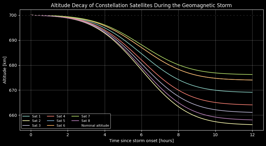
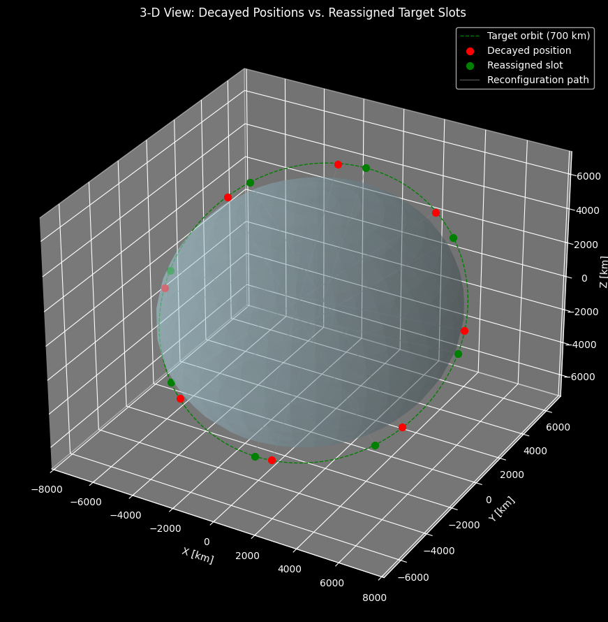
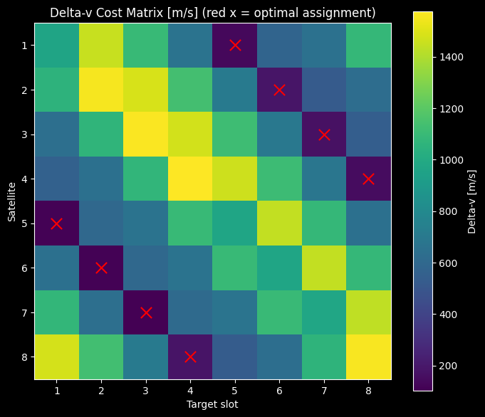
Section 7 — plots. Plot 7-1 shows the decay curves that motivated the whole problem. Plot 7-2 is the 3D centerpiece: Earth as a translucent sphere, the target orbital ring, the satellites’ decayed positions (red), and their reassigned target slots (green), connected by gray transfer lines — the inclination tilt makes the circular orbit render as a tilted ellipse in 3D space. Plots 7-3 and 7-4 break each satellite’s $\Delta v$ and time down into the Hohmann and phasing components. Plot 7-5 is the Pareto front itself, annotated with each $\alpha$ value. Plot 7-6 shows the full $8\times8$ cost matrix as a heatmap with the chosen assignment marked.
4. Reading the Results
The altitude-decay plot (7-1) should show eight curves starting at 700 km and dipping a few tens of kilometers during the storm’s peak around hour 6, then leveling off — each satellite losing a slightly different amount of altitude depending on its k_decay value.
The 3D plot (7-2) is where the optimization becomes tangible: because a Hohmann transfer always lands a satellite at the antipodal point of its orbit, you’ll likely notice that the Hungarian algorithm tends to assign each satellite to the slot roughly opposite its decayed position — phasing maneuvers then only need to make small corrections for the drift that accumulated during the storm, rather than large 45°+ corrections. This is a nice illustration of how orbital mechanics constraints (not just “distance”) shape the optimal assignment.
The fuel and time breakdown bars (7-3, 7-4) typically show the Hohmann transfer as a fairly uniform “base cost” across satellites (since all satellites need roughly the same altitude recovery), while the phasing contribution varies more — satellites with larger drift need either more $\Delta v$ or more phasing loops (more time) to correct it.
The Pareto front (7-5) is the headline result: moving from $\alpha=0$ (pure time minimization) to $\alpha=1$ (pure fuel minimization), total $\Delta v$ should decrease while total reconfiguration time increases — a smooth, monotonic trade-off curve. The $\alpha=0.5$ point (highlighted in red) represents a reasonable operational compromise, but an operator facing a tight propellant budget could shift toward $\alpha=1$, while one facing a tracking-window deadline could shift toward $\alpha=0$.
Finally, the cost-matrix heatmap (7-6) gives a sense of how “peaked” the assignment problem is — if the diagonal-ish band of low-cost entries is sharp, the optimal assignment is robust; if costs are more uniform, small changes in $\alpha$ could shuffle the assignment more freely.
5. Where to Go From Here
This model deliberately keeps things in a single orbital plane so that every maneuver is a simple in-plane burn. A natural extension is a true Walker constellation with multiple planes, where reassigning a satellite to a different plane requires an expensive plane-change burn — turning the cost matrix into something where cross-plane assignments are heavily penalized, and making the antipodal-swap pattern seen here even more dominant. Another extension is replacing the phenomenological decay model with a J2-perturbation-aware propagator, or replacing the “total time = sum over satellites” objective with a true makespan (max over satellites) objective for missions where all maneuvers happen in parallel — though that would require a more general solver than the Hungarian algorithm, since makespan is not a linear sum.