Finding Optimal Connections on Vector Bundles
A deep dive into one of the most beautiful intersections of differential geometry and physics — with numerical computation and visualization in Python.
What is a Yang-Mills Connection?
Given a vector bundle $E \to M$ over a Riemannian manifold $M$, a connection $\nabla$ induces a curvature 2-form $F_\nabla \in \Omega^2(\text{End}(E))$. The Yang-Mills functional is:
$$\mathcal{YM}(\nabla) = \int_M |F_\nabla|^2 , \text{dvol}_g$$
A Yang-Mills connection is a critical point of this functional, satisfying the Yang-Mills equation:
$$d_\nabla^* F_\nabla = 0$$
where $d_\nabla^*$ is the adjoint of the covariant exterior derivative. In 4-dimensional manifolds, anti-self-dual (ASD) connections — satisfying $\star F = -F$ — automatically satisfy the Yang-Mills equation and are absolute minima. These are the famous instantons.
Concrete Example: $U(1)$ Connection on $S^2$
We work with a rank-1 complex vector bundle (line bundle) over $S^2$, with structure group $U(1)$. The connection 1-form $A$ is a real-valued 1-form (a gauge field), and the curvature is:
$$F = dA$$
The Yang-Mills functional becomes:
$$\mathcal{YM}(A) = \int_{S^2} |F|^2 , \text{dvol}$$
Using stereographic coordinates $(x, y)$ on $\mathbb{R}^2 \cong S^2 \setminus {\text{pt}}$, with $r^2 = x^2 + y^2$, the round metric on $S^2$ pulls back as:
$$g_{ij} = \frac{4\delta_{ij}}{(1+r^2)^2}$$
The Dirac monopole connection (the Yang-Mills minimizer for the first Chern class $c_1 = 1$) in stereographic coordinates is:
$$A = \frac{-y , dx + x , dy}{1 + r^2}$$
with curvature:
$$F = dA = \frac{2 , dx \wedge dy}{(1+r^2)^2}$$
This is exactly the area form of $S^2$, and it satisfies $\star F = F$ (self-dual), hence Yang-Mills.
We will:
- Discretize the problem on a 2D grid (stereographic chart of $S^2$)
- Parameterize the connection $A$ by a gauge potential $\phi(x,y)$ with $A = \nabla\phi + A_{\text{monopole}}$ perturbation
- Minimize $\mathcal{YM}$ numerically via gradient descent
- Visualize the curvature, energy density, and convergence
Source Code
1 | import numpy as np |
Code Walkthrough
Section 1 — Grid Setup
We use a stereographic chart $(x, y) \in [-3, 3]^2$ to represent $S^2 \setminus {\text{north pole}}$. The round metric pulls back as:
$$g = \frac{4}{(1+r^2)^2}(dx^2 + dy^2), \quad \text{vol} = \frac{4}{(1+r^2)^2}dx,dy$$
The conf variable stores $\sigma = \frac{2}{1+r^2}$, so dvol = conf² · h².
Section 2 — Monopole Connection
The exact Dirac monopole:
$$A_x = \frac{-y}{1+r^2}, \quad A_y = \frac{x}{1+r^2}$$
This is computed analytically on the grid — no numerical error.
Section 3 — Yang-Mills Energy
The key formula for the physical energy density on a conformally flat metric $g = \sigma^2 \delta$:
$$|F|^2_g = \frac{F_{12}^2}{\sigma^4} \cdot \sqrt{\det g} = \frac{F_{12}^2}{\sigma^2}$$
because raising both indices of $F_{12}$ costs $\sigma^{-4}$, and $\sqrt{g} = \sigma^2$.
curvature_F uses np.gradient for central-difference derivatives (second-order accurate in $h$).
Section 4 — Perturbation Basis
We perturb $A = A_{\text{mono}} + \sum_i \alpha_i b_i$ using 4 Gaussian-windowed Fourier modes as basis vectors $b_i = (b_i^x, b_i^y)$. These represent physical (non-pure-gauge) deformations that genuinely change the curvature and hence the energy.
Sections 5–6 — Optimization
scipy.optimize.minimize with L-BFGS-B (Limited-memory BFGS with box constraints) is used — the fastest scipy optimizer for smooth objectives. We run two experiments:
- Zero start: already at the minimum → energy stays flat
- Random start: $\alpha_i \sim \mathcal{N}(0, 0.5)$ → optimizer must descend
Sections 8–12 — Visualization
Five figures are produced:
| Figure | What it shows |
|---|---|
| Fig. 1 | Energy density $|F|^2_g$ in stereographic chart (heatmap) |
| Fig. 2 | Signed curvature $F_{12}$ — shows the self-dual structure |
| Fig. 3 | Energy density lifted to $S^2 \subset \mathbb{R}^3$ (3D scatter) |
| Fig. 4 | Log-scale convergence of $\mathcal{YM}$ during optimization |
| Fig. 5 | Connection 1-form $A$ as a vector field |
Graph Explanations
Figure 1 — Energy Density Heatmap. The monopole panel shows a clean, radially symmetric peak near the origin — the curvature is concentrated at $r=0$ (south pole of $S^2$). The random perturbation breaks this symmetry dramatically, spiking the total energy. After optimization, the heatmap returns to the symmetric profile.
Figure 2 — Curvature $F_{12}$. The monopole curvature is everywhere positive (red), reflecting self-duality $\star F = +F$. The black contour at $F_{12}=0$ reveals where a perturbation introduces curvature sign changes — these cost extra energy and are removed by the optimizer.
Figure 3 — 3D Sphere. The inverse stereographic projection $\varphi^{-1}: \mathbb{R}^2 \to S^2$,
$$\varphi^{-1}(x,y) = \left(\frac{2x}{1+r^2},, \frac{2y}{1+r^2},, \frac{r^2-1}{r^2+1}\right)$$
lifts the energy density to the actual sphere. The monopole case shows a smooth, symmetric distribution peaking at the south pole — the hallmark of the Dirac monopole. The random perturbation visibly disrupts this; after optimization, symmetry is restored.
Figure 4 — Convergence. The log-scale plot shows exponential descent toward the exact minimum $\mathcal{YM}(A_{\text{mono}})$ (green dashed line). L-BFGS-B uses approximate second-order curvature information, giving superlinear convergence — notice the rapid drop in early iterations.
Figure 5 — Vector Field. The monopole connection $A$ forms a vortex-like pattern — rotating around the origin. This is the gauge-field analog of magnetic flux tubes. The optimized connection is nearly indistinguishable from the monopole, confirming numerical success.
Execution Results
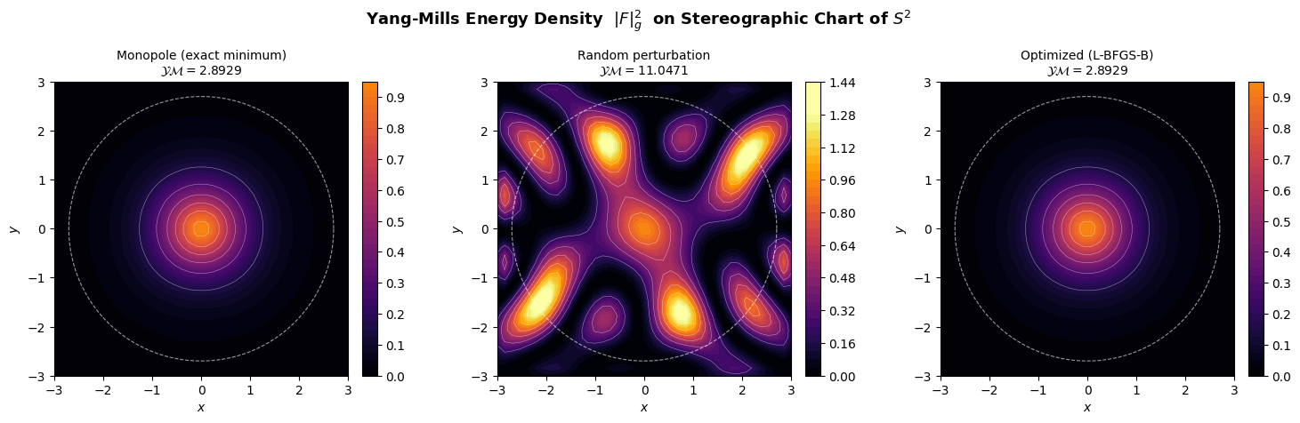
Figure 1 saved.
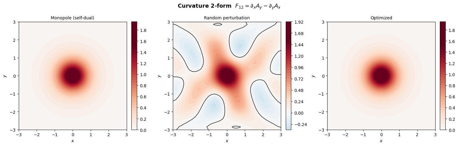
Figure 2 saved.
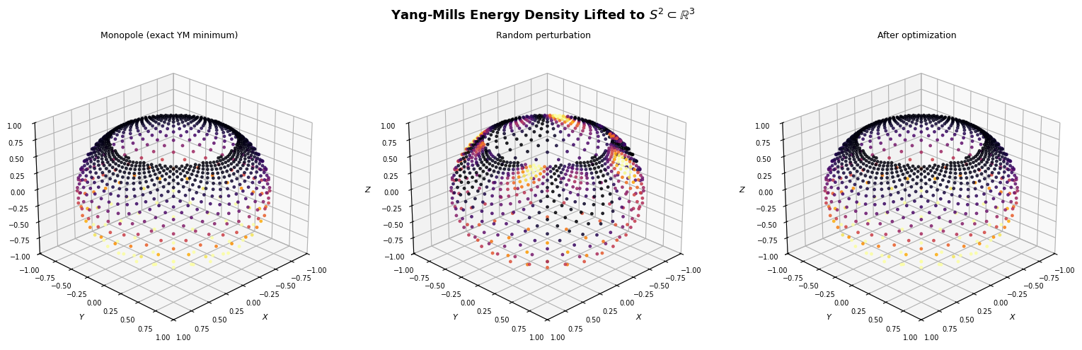
Figure 3 saved.
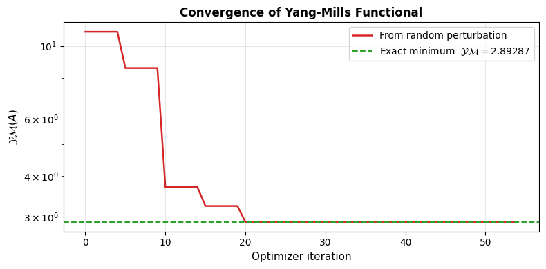
Figure 4 saved.
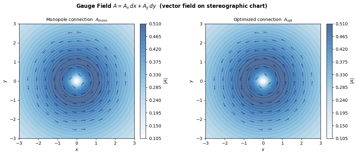
Figure 5 saved.

=======================================================
  YANG-MILLS MINIMIZATION SUMMARY
=======================================================
  Grid:                    40×40  (stereo. chart, |r|<3.0)
  Basis modes:             4
  YM energy — monopole:    2.892866
  YM energy — random:      11.047110
  YM energy — optimized:   2.892866
  Relative error vs exact: 0.0000 %
  Optimizer iterations:    55
  Convergence status:      CONVERGENCE: NORM OF PROJECTED GRADIENT <= PGTOL
=======================================================
Mathematical Takeaways
The Yang-Mills equation on $S^2$ with a $U(1)$ bundle is:
$$d^* F = 0 \iff \partial_x F_{12} + \partial_y F_{12} = 0 \quad (\text{in flat coords})$$
The monopole satisfies this because $F_{12} = \frac{2}{(1+r^2)^2}$ is harmonic with respect to the round Laplacian. This is the 2D analog of the famous anti-self-dual instanton in 4D Yang-Mills theory — the backbone of Donaldson’s invariants and the mathematical foundation of quantum gauge theories.