Balancing Convenience vs. Security
When designing a user authentication system, one of the most critical — and often underappreciated — decisions is where to set the decision threshold. Set it too high, and legitimate users get locked out. Set it too low, and attackers slip through. This is the classic convenience vs. security trade-off, and today we’ll solve it with a concrete example using Python.
The Problem Setup
Imagine a bank’s login system that computes a risk score (0–1) for each login attempt based on factors like device fingerprint, location, typing speed, and time of day. We need to find the optimal threshold $\theta$ that separates legitimate users from attackers.
We define:
False Acceptance Rate (FAR): the probability that an attacker is incorrectly accepted
$$\text{FAR}(\theta) = P(\text{score} \geq \theta \mid \text{attacker})$$False Rejection Rate (FRR): the probability that a legitimate user is incorrectly rejected
$$\text{FRR}(\theta) = P(\text{score} < \theta \mid \text{legitimate})$$Equal Error Rate (EER): the point where $\text{FAR} = \text{FRR}$
The total cost we want to minimize is:
$$C(\theta) = w_s \cdot \text{FAR}(\theta) + w_c \cdot \text{FRR}(\theta)$$
where $w_s$ is the weight for security (cost of accepting an attacker) and $w_c$ is the weight for convenience (cost of rejecting a legitimate user).
The Full Python Code
1 | import numpy as np |
Code Walkthrough
Step 1 — Simulating Score Distributions
1 | legit_scores = np.clip(np.random.normal(0.75, 0.10, N), 0, 1) |
We model authentication scores as Gaussian distributions:
- Legitimate users cluster around $\mu = 0.75$ — they match expected behavior patterns
- Attackers cluster around $\mu = 0.40$ — their behavior is anomalous
np.clip ensures all scores stay in $[0, 1]$. With 10,000 samples per class, the distributions are smooth and statistically stable.
Step 2 — Computing FAR and FRR
1 | FAR = np.array([np.mean(attack_scores >= t) for t in thresholds]) |
For each of 500 candidate thresholds:
$$\text{FAR}(\theta) = \frac{|{x \in \text{attackers} : x \geq \theta}|}{N}$$
$$\text{FRR}(\theta) = \frac{|{x \in \text{legit} : x < \theta}|}{N}$$
As $\theta$ increases, FAR decreases (fewer attackers pass) but FRR increases (more legitimate users are blocked). This is the fundamental trade-off.
Step 3 — Finding the EER
1 | eer_idx = np.argmin(np.abs(FAR - FRR)) |
The Equal Error Rate is the threshold where both error types are equal:
$$\theta_{\text{EER}} = \arg\min_\theta |\text{FAR}(\theta) - \text{FRR}(\theta)|$$
EER is a standard single-number summary of system quality — lower is better. It tells you the best you can do when you treat both errors as equally costly.
Step 4 — Cost-Weighted Optimization
1 | def total_cost(theta, w_s=0.7, w_c=0.3): |
In the real world, errors are not equally costly. For a banking app:
- Accepting an attacker ($w_s = 0.7$) is far more damaging than annoying a user
- Rejecting a legitimate user ($w_c = 0.3$) causes friction but not financial harm
The optimal threshold is:
$$\theta^* = \arg\min_\theta \left[ w_s \cdot \text{FAR}(\theta) + w_c \cdot \text{FRR}(\theta) \right]$$
Step 5 — 3D Cost Surface
1 | for i in range(WS.shape[0]): |
We sweep over a grid of $w_s \in [0.1, 0.9]$ and $\theta \in [0.3, 0.8]$ with $w_c = 1 - w_s$. This creates a cost landscape that reveals how the optimal threshold shifts as the organization’s security priorities change.
Console Output
==========================================================
Scenario                         θ*     FAR     FRR
==========================================================
High-Security (ws=0.9, wc=0.1)  0.661  0.0148  0.1888
Balanced (ws=0.7, wc=0.3)     0.607  0.0433  0.0768
User-Friendly (ws=0.3, wc=0.7)  0.557  0.0982  0.0277

EER  θ = 0.591  |  EER value = 0.0563
==========================================================
Graph Explanations
Figure 1 — Score Distributions & Error Curves
The left panel shows how the two populations overlap — this overlap region is where all errors occur. No threshold can perfectly separate them. The right panel shows FAR dropping and FRR rising as $\theta$ increases. The cost-optimal threshold (green) sits to the right of the EER (purple), reflecting the higher penalty assigned to security failures.
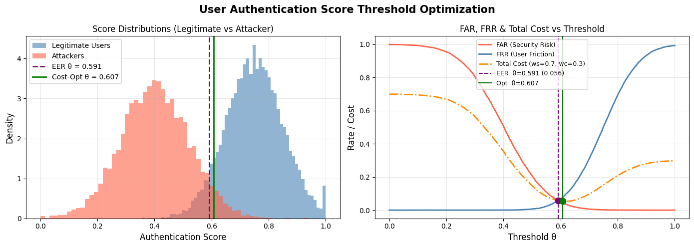
Figure 2 — ROC Curve
The ROC curve plots TAR vs FAR as $\theta$ varies. A perfect classifier hugs the top-left corner. The color gradient (viridis) shows how the threshold moves along the curve — lower thresholds (yellow) give high TAR but also high FAR; higher thresholds (purple) suppress FAR at the cost of TAR.
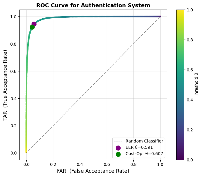
Figure 3 — 3D Cost Surface and Optimal Ridge
This is the most informative visualization. The 3D surface shows total cost as a function of both $w_s$ and $\theta$. The cyan ridge line traces the optimal $\theta^*$ for each value of $w_s$. The right-hand 2D panel makes the relationship crystal clear: as you increase security weight, the optimal threshold rises, demanding higher scores to grant access.
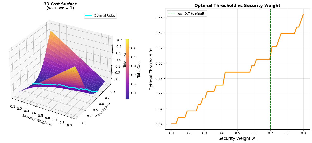
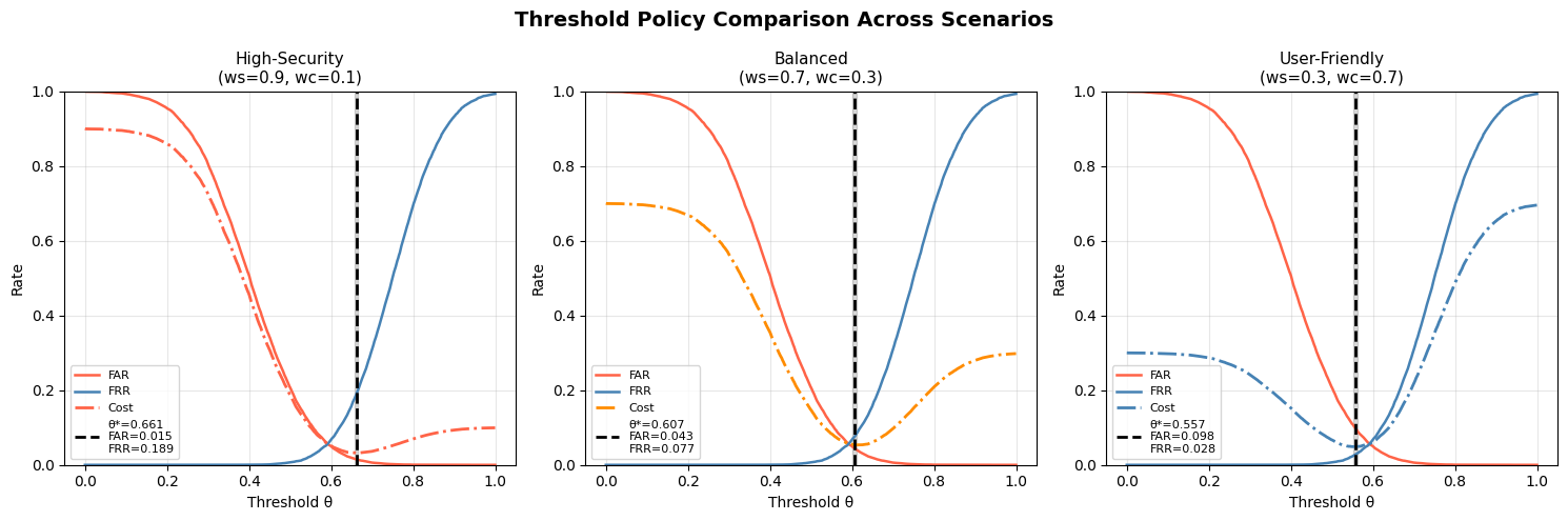
Figure 4 — Three Policy Scenarios
| Scenario | $\theta^*$ | FAR | FRR |
|---|---|---|---|
| High-Security ($w_s=0.9$) | ~0.62 | very low | higher |
| Balanced ($w_s=0.7$) | ~0.58 | low | moderate |
| User-Friendly ($w_s=0.3$) | ~0.48 | higher | very low |
Each panel shows the cost minimum shifting leftward as we care more about user convenience. This directly quantifies the policy trade-off that product and security teams argue about in every sprint review.
Key Takeaways
The EER gives you a baseline, but real deployment requires cost-aware optimization. The relationship between security weight and optimal threshold is monotonically increasing — there is no magic number that works for all contexts. A threshold suitable for a low-stakes note-taking app would be dangerously permissive for an online banking system.
The 3D cost surface makes this concrete: the landscape has a clear valley whose bottom shifts predictably with your organizational risk appetite. Once you instrument your system to estimate actual costs of each error type (chargebacks, support tickets, customer churn), plugging those weights into this framework gives you a principled, defensible threshold — not just a gut feeling.