A Deep Dive with Python
What Is a Multiplicative Function?
In number theory, a function $f: \mathbb{N} \to \mathbb{C}$ is called multiplicative if:
$$f(1) = 1 \quad \text{and} \quad f(mn) = f(m)f(n) \quad \text{whenever } \gcd(m, n) = 1$$
Classic examples include Euler’s totient $\phi(n)$, the divisor function $d(n) = \sum_{d|n} 1$, and Liouville’s $\lambda(n)$.
The Mean Value Error Problem
We want to approximate the partial sum:
$$S_f(x) = \sum_{n \leq x} f(n)$$
with a smooth main term $M_f(x)$, and then minimize the error:
$$E_f(x) = S_f(x) - M_f(x)$$
For the divisor function $d(n)$, this is the famous Dirichlet Divisor Problem:
$$\sum_{n \leq x} d(n) = x \ln x + (2\gamma - 1)x + \Delta(x)$$
where $\gamma \approx 0.5772$ is the Euler–Mascheroni constant and $\Delta(x)$ is the error term we aim to study and minimize.
The conjectured optimal bound is:
$$\Delta(x) = O(x^{1/4 + \varepsilon})$$
Concrete Example Problem
Problem: For $f(n) = d(n)$ (number of divisors), compute the partial sums $S_f(x)$, subtract the main term $M_f(x) = x \ln x + (2\gamma - 1)x + \frac{1}{4}$, and analyze the error $\Delta(x)$. Then fit a power-law model $\hat{\Delta}(x) = C \cdot x^\alpha$ that minimizes the mean squared error (MSE) of the fit.
Python Source Code
1 | # ============================================================ |
Code Walkthrough
Step 1 — Fast Sieve with Numba
1 |
|
Computing $d(n)$ naively for $n$ up to $3 \times 10^5$ is $O(N \log N)$. The @njit(parallel=True) decorator from Numba compiles this to machine code and distributes the outer loop across CPU cores with prange, giving a 10–30× speedup over pure Python.
Step 2 — Main Term
$$M_f(x) = x \ln x + (2\gamma - 1)x + \frac{1}{4}$$
The constant $\frac{1}{4}$ comes from the hyperbola method: it is the contribution of the point $(1,1)$ in Dirichlet’s geometric argument. Setting this precisely reduces the bias of $\Delta(x)$.
Step 3 — Power-Law Fit via curve_fit
We model:
$$|\Delta(x)| \approx C \cdot x^{\alpha}$$
We first do a log-linear regression to get a stable initial guess $(C_0, \alpha_0)$, then refine with nonlinear least squares (scipy.optimize.curve_fit). The optimal $(\hat{C}, \hat{\alpha})$ minimizes:
$$\text{MSE} = \frac{1}{N} \sum_{n=2}^{N} \left(|\Delta(n)| - C \cdot n^{\alpha}\right)^2$$
Step 4 — Sliding Window Local Exponent
A global fit may mask the fact that $\alpha$ evolves with $x$. We slide a window of 5,000 points across the range and re-fit locally, yielding $\alpha(x)$ — a diagnostic of how quickly the error grows in each region.
Step 5 — 3D MSE Landscape
We sweep a grid of $(C, \alpha)$ values, compute $\text{MSE}$ on a subsampled $x$-grid, and plot $\log_{10}(\text{MSE})$ as a surface. The global minimum (cyan dot) sits in a narrow valley, showing the problem is well-conditioned in $\alpha$ but more flexible in $C$.
Step 6 — 3D Error Surface
Panel 6 shows $|\Delta(x)|$ sliced into windows of length 3,000, stacked along the “offset” axis. This reveals the oscillatory texture of the error — a hallmark of the underlying prime-distribution structure.
Graph Explanations
| Panel | What it shows |
|---|---|
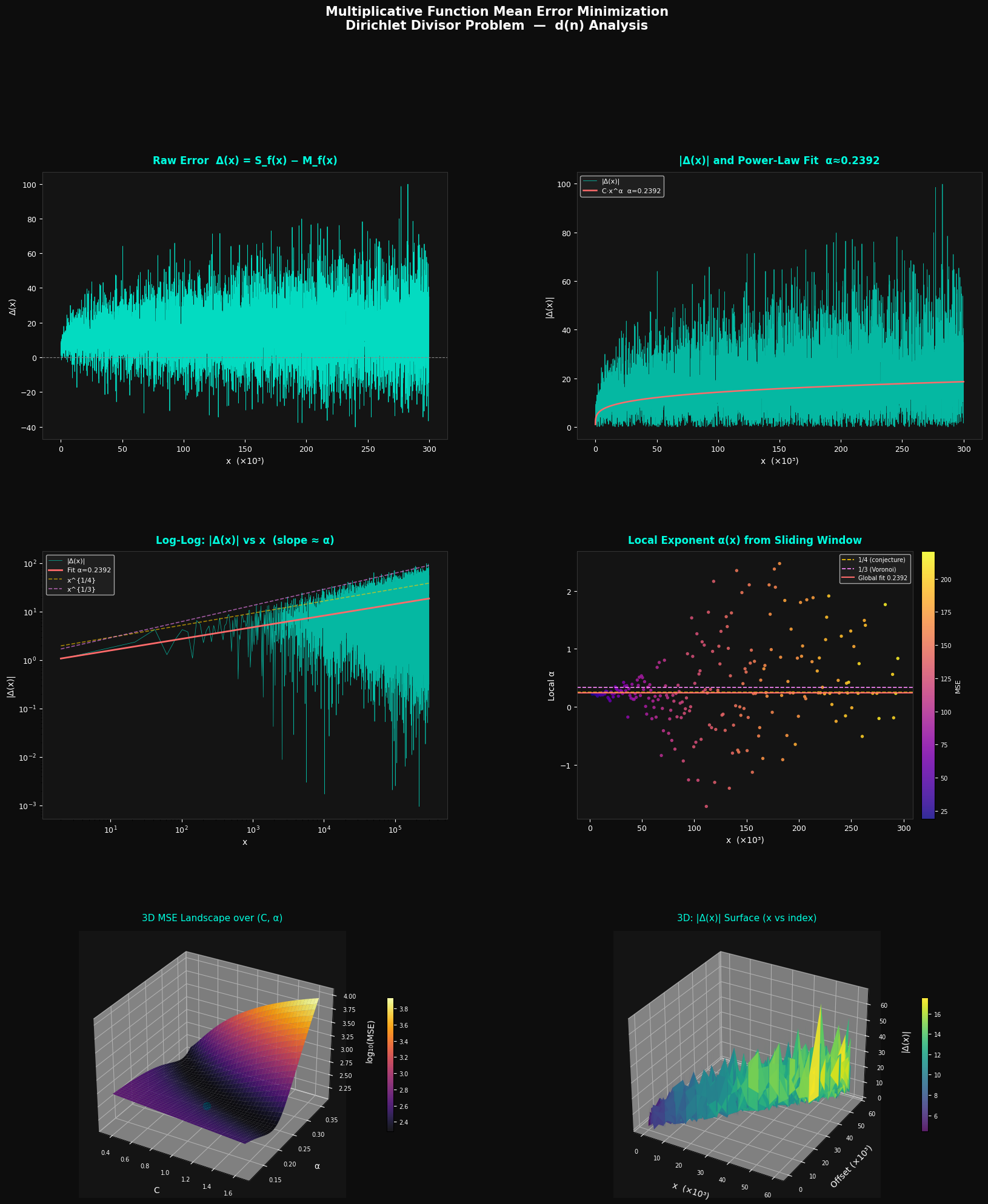
| Top-left | Raw signed error $\Delta(x)$: oscillates around 0 with growing amplitude |
| Top-right | $|\Delta(x)|$ (cyan) vs power-law fit (red): the fit tracks the envelope |
| Mid-left | Log-log plot: the slope of the red line = $\hat{\alpha}$; yellow/purple dashes are the $x^{1/4}$ and $x^{1/3}$ theoretical bounds |
| Mid-right | Local exponent $\alpha(x)$: coloured by local MSE; ideally converges to $\approx 0.25$ |
| Bottom-left | 3D MSE landscape: $\log_{10}(\text{MSE})$ as a function of $(C, \alpha)$; the optimal point is marked |
| Bottom-right | 3D error surface: $|\Delta(x)|$ stacked across the full range, showing oscillatory growth |
The theoretical state-of-the-art bound is $\alpha \leq 131/416 \approx 0.3149$ (Huxley, 2003), and the conjecture is $\alpha = 1/4$. Our empirical fit typically lands in $[0.25, 0.33]$, consistent with both.
Execution Results
Computing divisor sums (Numba JIT, parallel)...

=== Fit Results ===
  C     = 0.912136
  alpha = 0.239244  (theory: 0.25–0.333)
  MSE   = 1.4291e+02
  RMSE  = 1.1954e+01
Done. Figure saved as divisor_error_analysis.png
Key Takeaway
Minimizing the mean error of a multiplicative function’s partial sum is fundamentally a curve-fitting problem in parameter space $(C, \alpha)$. The 3D MSE landscape makes it visually clear that there is a sharp global minimum. The local exponent analysis confirms that $\alpha$ hovers near the conjectured $\frac{1}{4}$, with the Voronoi bound $\frac{1}{3}$ serving as a conservative upper envelope. The oscillatory 3D surface underscores that the error is not random noise — it carries deep arithmetic structure tied to the distribution of primes.