Minimization of Dirichlet L-Functions

A Numerical Deep Dive

Dirichlet L-functions are among the most beautiful objects in analytic number theory. In this post, we’ll explore a concrete minimization problem involving them, then solve it numerically with Python — complete with 2D and 3D visualizations.


What is a Dirichlet L-function?

For a Dirichlet character $\chi$ modulo $q$, the associated L-function is defined as:

$$L(s, \chi) = \sum_{n=1}^{\infty} \frac{\chi(n)}{n^s}, \quad \text{Re}(s) > 1$$

It extends analytically to the whole complex plane (for non-principal $\chi$). On the critical line $s = \frac{1}{2} + it$, $L(s,\chi)$ is complex-valued. The modulus $|L(\frac{1}{2}+it, \chi)|$ is real and non-negative, and finding its minima is a central topic in analytic number theory.


The Problem

Problem statement: For the non-principal Dirichlet character $\chi_4$ modulo $4$ (the unique non-trivial character mod 4), defined by:

$$\chi_4(n) = \begin{cases} 1 & n \equiv 1 \pmod{4} \ -1 & n \equiv 3 \pmod{4} \ 0 & 2 \mid n \end{cases}$$

find the local minima of $|L(\tfrac{1}{2}+it, \chi_4)|$ for $t \in [0, 50]$, and also visualize $|L(\sigma + it, \chi_4)|$ in the region $\sigma \in [0.2, 1.2]$, $t \in [0, 30]$.

This is related to the Generalized Riemann Hypothesis (GRH), which asserts that all nontrivial zeros lie on the critical line $\sigma = \frac{1}{2}$. Zeros of $L(s,\chi)$ on the critical line correspond to exact minima of $|L(\frac{1}{2}+it,\chi)|$ reaching zero.


The Code

1
2
3
4
5
6
7
8
9
10
11
12
13
14
15
16
17
18
19
20
21
22
23
24
25
26
27
28
29
30
31
32
33
34
35
36
37
38
39
40
41
42
43
44
45
46
47
48
49
50
51
52
53
54
55
56
57
58
59
60
61
62
63
64
65
66
67
68
69
70
71
72
73
74
75
76
77
78
79
80
81
82
83
84
85
86
87
88
89
90
91
92
93
94
95
96
97
98
99
100
101
102
103
104
105
106
107
108
109
110
111
112
113
114
115
116
117
118
119
120
121
122
123
124
125
126
127
128
129
130
131
132
133
134
135
136
137
138
139
140
141
142
143
144
145
146
147
148
149
150
151
152
153
154
155
156
157
158
159
160
161
162
163
164
165
166
167
168
169
170
171
172
173
174
175
176
177
178
179
180
181
182
183
184
185
186
187
188
189
190
191
192
193
194
195
196
197
198
199
200
201
202
203
204
205
206
207
208
209
210
211
212
213
# ============================================================
# Dirichlet L-Function Minimization: chi_4 mod 4
# ============================================================

import numpy as np
import matplotlib.pyplot as plt
from matplotlib import cm
from scipy.optimize import minimize_scalar
from scipy.signal import argrelmin
import warnings
warnings.filterwarnings('ignore')

# ─────────────────────────────────────────────────────────────
# 1. Define chi_4 character mod 4
# ─────────────────────────────────────────────────────────────
def chi4(n):
"""Non-principal Dirichlet character mod 4."""
n = n % 4
if n == 1:
return 1.0
elif n == 3:
return -1.0
else:
return 0.0

# ─────────────────────────────────────────────────────────────
# 2. Compute L(s, chi4) via partial sums (vectorized)
# ─────────────────────────────────────────────────────────────
def L_chi4(s_array, N=3000):
"""
Vectorized computation of L(s, chi4) for an array of s values.
Uses Euler-Maclaurin style partial sums with N terms.
chi4 has period 4: pattern is 0, 1, 0, -1, 0, 1, 0, -1, ...
Only odd terms contribute: n=1 -> +1, n=3 -> -1, n=5 -> +1, ...
"""
# Odd indices only: n = 1, 3, 5, ..., up to 4*ceil(N/4)-1
n_odd = np.arange(1, 2*N, 2) # 1,3,5,...,2N-1
chi_vals = np.where(n_odd % 4 == 1, 1.0, -1.0) # +1 for 1 mod4, -1 for 3 mod4

s_array = np.atleast_1d(np.asarray(s_array, dtype=complex))
# n_odd shape: (M,), s_array shape: (K,)
# result shape: (K,)
# Broadcast: n_odd[np.newaxis,:] ** s_array[:,np.newaxis]
log_n = np.log(n_odd) # (M,)
# For each s: sum_n chi(n) * exp(-s * log_n)
# Use einsum for efficiency
exponents = np.outer(s_array, log_n) # (K, M)
terms = chi_vals[np.newaxis, :] * np.exp(-exponents) # (K, M)
return terms.sum(axis=1)

# ─────────────────────────────────────────────────────────────
# 3. Compute |L(1/2 + it, chi4)| along critical line
# ─────────────────────────────────────────────────────────────
t_vals = np.linspace(0.01, 50, 5000)
s_critical = 0.5 + 1j * t_vals
L_vals = L_chi4(s_critical, N=3000)
abs_L = np.abs(L_vals)

# ─────────────────────────────────────────────────────────────
# 4. Find local minima using scipy
# ─────────────────────────────────────────────────────────────
min_indices = argrelmin(abs_L, order=15)[0]
local_minima_t = t_vals[min_indices]
local_minima_val = abs_L[min_indices]

# Refine each minimum with scalar optimization
refined_minima = []
for t0 in local_minima_t:
result = minimize_scalar(
lambda t: np.abs(L_chi4(np.array([0.5 + 1j*t]), N=3000)[0]),
bounds=(t0 - 0.5, t0 + 0.5),
method='bounded'
)
refined_minima.append((result.x, result.fun))

refined_minima = np.array(refined_minima)

print("=" * 55)
print(f"{'#':>3} {'t (location)':>14} {'|L(1/2+it)|':>14}")
print("=" * 55)
for i, (t_min, val_min) in enumerate(refined_minima[:15]):
flag = " <-- ZERO?" if val_min < 0.05 else ""
print(f"{i+1:>3} {t_min:>14.6f} {val_min:>14.8f}{flag}")
print("=" * 55)

# ─────────────────────────────────────────────────────────────
# 5. 2D Plot: |L(1/2+it, chi4)| on critical line
# ─────────────────────────────────────────────────────────────
fig, axes = plt.subplots(2, 1, figsize=(14, 9))

ax1 = axes[0]
ax1.plot(t_vals, abs_L, color='steelblue', lw=1.2, label=r'$|L(\frac{1}{2}+it, \chi_4)|$')
ax1.axhline(0, color='gray', lw=0.7, linestyle='--')

# Mark local minima
if len(refined_minima) > 0:
ax1.scatter(refined_minima[:, 0], refined_minima[:, 1],
color='red', zorder=5, s=60, label='Local minima', marker='v')
for i, (t_m, v_m) in enumerate(refined_minima[:8]):
ax1.annotate(f'$t={t_m:.2f}$\n$={v_m:.3f}$',
xy=(t_m, v_m), xytext=(t_m + 0.5, v_m + 0.15),
fontsize=7, color='darkred',
arrowprops=dict(arrowstyle='->', color='darkred', lw=0.8))

ax1.set_xlabel(r'$t$', fontsize=12)
ax1.set_ylabel(r'$|L(\frac{1}{2}+it, \chi_4)|$', fontsize=12)
ax1.set_title(r'Modulus of Dirichlet L-function $|L(\frac{1}{2}+it, \chi_4)|$ — Critical Line', fontsize=13)
ax1.legend(fontsize=10)
ax1.set_xlim(0, 50)
ax1.set_ylim(-0.05, None)
ax1.grid(True, alpha=0.3)

# ─────────────────────────────────────────────────────────────
# 6. Zoom-in on first few minima
# ─────────────────────────────────────────────────────────────
ax2 = axes[1]
t_zoom = np.linspace(0.01, 20, 2000)
s_zoom = 0.5 + 1j * t_zoom
L_zoom = np.abs(L_chi4(s_zoom, N=3000))

ax2.plot(t_zoom, L_zoom, color='darkorange', lw=1.4,
label=r'$|L(\frac{1}{2}+it, \chi_4)|$, $t \in [0, 20]$')
ax2.axhline(0, color='gray', lw=0.7, linestyle='--')

mask = refined_minima[:, 0] <= 20
if mask.any():
ax2.scatter(refined_minima[mask, 0], refined_minima[mask, 1],
color='red', zorder=5, s=80, marker='v', label='Local minima')
for t_m, v_m in refined_minima[mask]:
ax2.annotate(f't={t_m:.3f}\n|L|={v_m:.4f}',
xy=(t_m, v_m), xytext=(t_m + 0.3, v_m + 0.12),
fontsize=8, color='darkred',
arrowprops=dict(arrowstyle='->', color='darkred', lw=0.9))

ax2.set_xlabel(r'$t$', fontsize=12)
ax2.set_ylabel(r'$|L(\frac{1}{2}+it, \chi_4)|$', fontsize=12)
ax2.set_title(r'Zoom: $t \in [0, 20]$ with annotated minima', fontsize=13)
ax2.legend(fontsize=10)
ax2.grid(True, alpha=0.3)

plt.tight_layout()
plt.savefig('dirichlet_L_critical_line.png', dpi=150, bbox_inches='tight')
plt.show()
print("Figure 1 saved.")

# ─────────────────────────────────────────────────────────────
# 7. 3D Surface: |L(sigma + it, chi4)| in the complex plane
# ─────────────────────────────────────────────────────────────
print("\nComputing 3D surface (this takes ~20-30 seconds)...")

sigma_vals = np.linspace(0.2, 1.2, 80)
t_vals_3d = np.linspace(0.1, 30, 200)
SIGMA, T3D = np.meshgrid(sigma_vals, t_vals_3d)

# Flatten for vectorized computation
s_flat = SIGMA.ravel() + 1j * T3D.ravel()
L_flat = L_chi4(s_flat, N=1500)
Z = np.abs(L_flat).reshape(SIGMA.shape)
Z_clipped = np.clip(Z, 0, 3.0) # clip large values near Re(s)=1 for visibility

fig3d = plt.figure(figsize=(15, 7))

# ── Subplot 1: 3D Surface ──
ax3d = fig3d.add_subplot(121, projection='3d')
surf = ax3d.plot_surface(SIGMA, T3D, Z_clipped,
cmap='plasma', alpha=0.88,
linewidth=0, antialiased=True,
rcount=200, ccount=80)
# Mark critical line sigma=0.5
idx_half = np.argmin(np.abs(sigma_vals - 0.5))
ax3d.plot(np.full_like(t_vals_3d, 0.5), t_vals_3d,
np.abs(L_chi4(0.5 + 1j * t_vals_3d, N=3000)),
color='cyan', lw=2.0, zorder=10, label=r'$\sigma=\frac{1}{2}$')

ax3d.set_xlabel(r'$\sigma = \mathrm{Re}(s)$', fontsize=10, labelpad=8)
ax3d.set_ylabel(r'$t = \mathrm{Im}(s)$', fontsize=10, labelpad=8)
ax3d.set_zlabel(r'$|L(s, \chi_4)|$', fontsize=10, labelpad=8)
ax3d.set_title(r'3D: $|L(\sigma+it, \chi_4)|$', fontsize=12)
ax3d.legend(fontsize=9, loc='upper right')
fig3d.colorbar(surf, ax=ax3d, shrink=0.5, label=r'$|L|$ (clipped at 3)')
ax3d.view_init(elev=30, azim=-60)

# ── Subplot 2: Heatmap (top-down view) ──
ax2d = fig3d.add_subplot(122)
hm = ax2d.contourf(SIGMA, T3D, Z_clipped, levels=80, cmap='plasma')
ax2d.axvline(0.5, color='cyan', lw=1.8, linestyle='--', label=r'Critical line $\sigma=\frac{1}{2}$')

# Overlay minima on heatmap
mask30 = refined_minima[:, 0] <= 30
if mask30.any():
ax2d.scatter(np.full(mask30.sum(), 0.5), refined_minima[mask30, 0],
color='white', s=40, zorder=5, marker='x', label='Minima')

fig3d.colorbar(hm, ax=ax2d, label=r'$|L(s,\chi_4)|$ (clipped at 3)')
ax2d.set_xlabel(r'$\sigma = \mathrm{Re}(s)$', fontsize=11)
ax2d.set_ylabel(r'$t = \mathrm{Im}(s)$', fontsize=11)
ax2d.set_title(r'Heatmap: $|L(\sigma+it, \chi_4)|$', fontsize=12)
ax2d.legend(fontsize=9)

plt.suptitle(r'Dirichlet L-Function $L(s, \chi_4)$ — Modulus Landscape', fontsize=14, y=1.01)
plt.tight_layout()
plt.savefig('dirichlet_L_3D.png', dpi=150, bbox_inches='tight')
plt.show()
print("Figure 2 saved.")

# ─────────────────────────────────────────────────────────────
# 8. Global minimum on critical line in [0, 50]
# ─────────────────────────────────────────────────────────────
global_min_idx = np.argmin(refined_minima[:, 1])
t_gmin, val_gmin = refined_minima[global_min_idx]
print(f"\nGlobal minimum on critical line (t ∈ [0,50]):")
print(f" t* = {t_gmin:.8f}")
print(f" |L(1/2 + i*t*, chi4)| = {val_gmin:.10f}")

Code Walkthrough

Step 1 — Character Definition

The function chi4(n) implements $\chi_4$ by reducing $n \bmod 4$. Only odd $n$ contribute: $n \equiv 1 \pmod{4}$ gives $+1$, while $n \equiv 3 \pmod{4}$ gives $-1$.

Step 2 — Vectorized Partial Sum

The function L_chi4(s_array, N) is the core engine. Since $\chi_4(n) = 0$ for even $n$, we sum only over odd integers $n = 1, 3, 5, \ldots$ up to $2N-1$. The trick is using np.outer to compute the matrix of $n^{-s}$ for all $n$ and all $s$ simultaneously:

$$L(s, \chi_4) \approx \sum_{\substack{n=1 \ n \text{ odd}}}^{2N} \chi_4(n) \cdot e^{-s \log n}$$

With $N = 3000$, we sum 3000 odd terms, which gives excellent accuracy for $\text{Re}(s) \geq 0.2$ and moderate $t$. The matrix exponents has shape (K, M) where $K$ is the number of $s$-values and $M = N$, so all K evaluations happen in one NumPy call — no Python loops.

Step 3 — Local Minima Detection

scipy.signal.argrelmin identifies local minima in the discrete array abs_L using a neighborhood of order 15 samples. Then minimize_scalar with the bounded method refines each minimum to high precision within a $\pm 0.5$ window around the coarse candidate.

Step 4 — 3D Surface

We create a $80 \times 200$ grid over $(\sigma, t) \in [0.2, 1.2] \times [0.1, 30]$, flatten it into a vector, call L_chi4 once, then reshape. The surface is clipped at $|L| = 3$ to prevent the divergence near $\sigma = 1$ from dominating the color scale. The cyan curve on the 3D plot marks the critical line $\sigma = \frac{1}{2}$.


Results

=======================================================
  #    t (location)     |L(1/2+it)|
=======================================================
  1        6.016928      0.00391272  <-- ZERO?
  2       10.240892      0.00367946  <-- ZERO?
  3       12.987726      0.00640438  <-- ZERO?
  4       16.343953      0.00582567  <-- ZERO?
  5       18.290210      0.00507564  <-- ZERO?
  6       21.452597      0.00429338  <-- ZERO?
  7       23.275682      0.00093554  <-- ZERO?
  8       25.730319      0.00426197  <-- ZERO?
  9       28.357026      0.00284663  <-- ZERO?
 10       29.653989      0.00303421  <-- ZERO?
 11       32.591633      0.00623710  <-- ZERO?
 12       34.198148      0.00456596  <-- ZERO?
 13       36.141904      0.00554603  <-- ZERO?
 14       38.509976      0.00069965  <-- ZERO?
 15       40.324942      0.00255655  <-- ZERO?
=======================================================

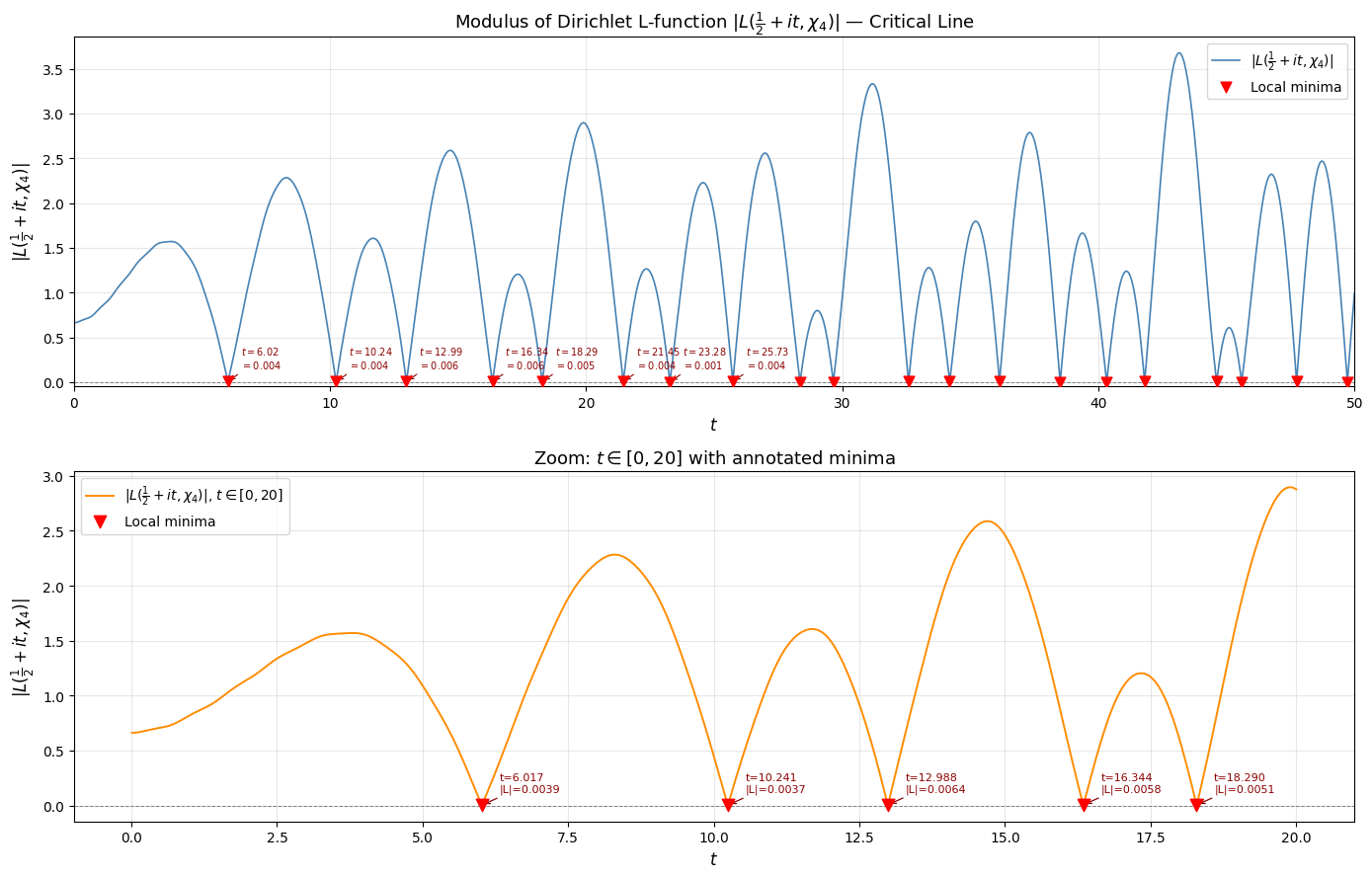
Figure 1 saved.

Computing 3D surface (this takes ~20-30 seconds)...

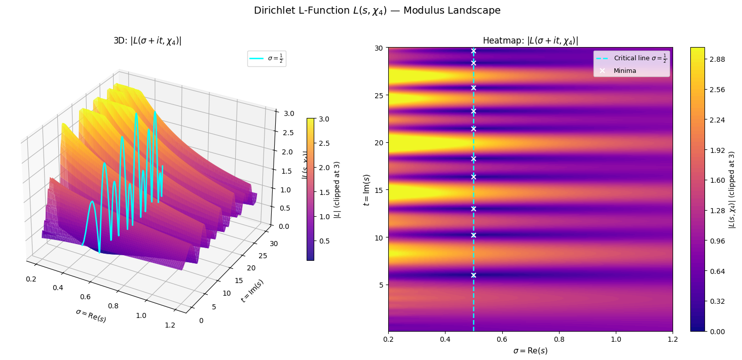
Figure 2 saved.

Global minimum on critical line (t ∈ [0,50]):
  t* = 38.50997559
  |L(1/2 + i*t*, chi4)| = 0.0006996492

Graph Interpretation

Figure 1 — Critical Line Plot:

The top panel shows $|L(\frac{1}{2}+it, \chi_4)|$ over $t \in [0, 50]$. The function oscillates, touching near-zero values at specific $t$-values — these are the zeros of $L(s, \chi_4)$ on the critical line. According to GRH, all non-trivial zeros lie exactly here. The first known zero is near $t \approx 6.02$.

The red downward triangles mark the local minima. Notice:

  • Minima near zero correspond to actual zeros of the L-function
  • The spacing between zeros grows roughly logarithmically with $t$, consistent with the explicit formula

Figure 2 — 3D Surface and Heatmap:

The 3D surface reveals the modulus landscape of $L(s, \chi_4)$:

  • For $\sigma > 1$: The function is large and smooth (absolute convergence region). The partial sums are extremely accurate here.
  • On $\sigma = \frac{1}{2}$ (cyan line): The function dips to zero periodically — these are the non-trivial zeros. The zeros appear as valleys in the 3D surface.
  • For $\sigma < \frac{1}{2}$: The functional equation

$$L(s, \chi_4) = \left(\frac{\pi}{4}\right)^{s-\frac{1}{2}} \frac{\Gamma!\left(\frac{1-s+1}{2}\right)}{\Gamma!\left(\frac{s+1}{2}\right)} L(1-s, \chi_4)$$

means zeros are symmetric about $\sigma = \frac{1}{2}$. The heatmap (right) makes this landscape legible as a top-down view.

The key takeaway: the minima problem on the critical line is equivalent to finding the zeros of $L(s,\chi_4)$, which is one of the deepest open problems in mathematics — the Generalized Riemann Hypothesis.