Solving the Staff Shift Assignment Problem with Python

What is the Staff Shift Assignment Problem?

The Staff Shift Assignment Problem is a classic combinatorial optimization problem. Given a set of employees and shifts, the goal is to assign workers to shifts while satisfying various constraints — minimum staffing levels, employee availability, labor regulations, and fairness requirements.


Problem Formulation

Let’s define the variables:

  • Let $E = {e_1, e_2, \ldots, e_m}$ be the set of employees
  • Let $S = {s_1, s_2, \ldots, s_n}$ be the set of shifts
  • Let $x_{ij} \in {0, 1}$ be a binary decision variable where $x_{ij} = 1$ if employee $i$ is assigned to shift $j$

Objective Function — minimize total cost:

$$\min \sum_{i \in E} \sum_{j \in S} c_{ij} \cdot x_{ij}$$

Subject to:

Minimum staffing per shift:
$$\sum_{i \in E} x_{ij} \geq d_j \quad \forall j \in S$$

Maximum shifts per employee per week:
$$\sum_{j \in S} x_{ij} \leq W_{max} \quad \forall i \in E$$

Availability constraint (employee $i$ cannot work shift $j$ if unavailable):
$$x_{ij} \leq a_{ij} \quad \forall i \in E, \forall j \in S$$


Concrete Example

We have 8 employees and 6 shifts over one week:

Shift Time Required Staff
Morning Mon 6:00–14:00 3
Afternoon Mon 14:00–22:00 2
Night Mon 22:00–6:00 1
Morning Fri 6:00–14:00 3
Afternoon Fri 14:00–22:00 2
Night Fri 22:00–6:00 1

Each employee has individual availability and a max of 3 shifts per week. We use PuLP to solve this Integer Linear Program.


Full Source Code

1
2
3
4
5
6
7
8
9
10
11
12
13
14
15
16
17
18
19
20
21
22
23
24
25
26
27
28
29
30
31
32
33
34
35
36
37
38
39
40
41
42
43
44
45
46
47
48
49
50
51
52
53
54
55
56
57
58
59
60
61
62
63
64
65
66
67
68
69
70
71
72
73
74
75
76
77
78
79
80
81
82
83
84
85
86
87
88
89
90
91
92
93
94
95
96
97
98
99
100
101
102
103
104
105
106
107
108
109
110
111
112
113
114
115
116
117
118
119
120
121
122
123
124
125
126
127
128
129
130
131
132
133
134
135
136
137
138
139
140
141
142
143
144
145
146
147
148
149
150
151
152
153
154
155
156
157
158
159
160
161
162
163
164
165
166
167
168
169
170
171
172
173
174
175
176
177
178
179
180
181
182
183
184
185
186
187
188
189
190
191
192
193
194
195
196
197
198
199
200
201
202
203
204
205
206
207
208
# ============================================================
# Staff Shift Assignment Problem
# Solver: PuLP (Integer Linear Programming)
# ============================================================

!pip install pulp -q

import pulp
import numpy as np
import matplotlib.pyplot as plt
import matplotlib.patches as mpatches
from mpl_toolkits.mplot3d import Axes3D
import matplotlib.cm as cm
import warnings
warnings.filterwarnings('ignore')

# ── 1. Problem Data ──────────────────────────────────────────
np.random.seed(42)

employees = [f"Emp_{i+1}" for i in range(8)]
shifts = ["Mon_Morning", "Mon_Afternoon", "Mon_Night",
"Fri_Morning", "Fri_Afternoon", "Fri_Night"]

n_emp = len(employees)
n_shift = len(shifts)

# Required staff per shift
required = {"Mon_Morning": 3, "Mon_Afternoon": 2, "Mon_Night": 1,
"Fri_Morning": 3, "Fri_Afternoon": 2, "Fri_Night": 1}

# Cost matrix (e.g. overtime preference, skill match)
# Lower cost = more preferred assignment
cost = {
(e, s): np.random.randint(1, 10)
for e in employees for s in shifts
}

# Availability matrix (1 = available, 0 = not available)
availability = {
("Emp_1","Mon_Night"):0, ("Emp_1","Fri_Night"):0,
("Emp_2","Mon_Morning"):0,
("Emp_3","Fri_Night"):0,
("Emp_4","Mon_Night"):0, ("Emp_4","Fri_Morning"):0,
("Emp_5","Mon_Afternoon"):0,
("Emp_6","Fri_Night"):0, ("Emp_6","Mon_Night"):0,
("Emp_7","Mon_Morning"):0,
("Emp_8","Fri_Afternoon"):0,
}
# Default availability = 1
avail = {(e, s): availability.get((e, s), 1)
for e in employees for s in shifts}

MAX_SHIFTS_PER_EMPLOYEE = 3

# ── 2. Build ILP Model ────────────────────────────────────────
prob = pulp.LpProblem("ShiftAssignment", pulp.LpMinimize)

# Decision variables
x = pulp.LpVariable.dicts("assign",
[(e, s) for e in employees for s in shifts],
cat="Binary")

# Objective: minimize total cost
prob += pulp.lpSum(cost[e, s] * x[e, s]
for e in employees for s in shifts)

# Constraint 1: meet minimum staffing requirement
for s in shifts:
prob += pulp.lpSum(x[e, s] for e in employees) >= required[s], f"min_staff_{s}"

# Constraint 2: max shifts per employee
for e in employees:
prob += pulp.lpSum(x[e, s] for s in shifts) <= MAX_SHIFTS_PER_EMPLOYEE, f"max_shift_{e}"

# Constraint 3: availability
for e in employees:
for s in shifts:
prob += x[e, s] <= avail[e, s], f"avail_{e}_{s}"

# ── 3. Solve ──────────────────────────────────────────────────
solver = pulp.PULP_CBC_CMD(msg=0)
status = prob.solve(solver)

print(f"Status : {pulp.LpStatus[prob.status]}")
print(f"Total Cost : {int(pulp.value(prob.objective))}")
print()

# ── 4. Extract Results ────────────────────────────────────────
assign_matrix = np.zeros((n_emp, n_shift), dtype=int)

print(f"{'Employee':<14}", end="")
for s in shifts:
print(f"{s:<17}", end="")
print()
print("-" * (14 + 17 * n_shift))

for i, e in enumerate(employees):
print(f"{e:<14}", end="")
for j, s in enumerate(shifts):
val = int(pulp.value(x[e, s]))
assign_matrix[i, j] = val
symbol = "✓" if val == 1 else "."
print(f"{symbol:<17}", end="")
total = assign_matrix[i].sum()
print(f" (total={total})")

print()
print("Staffing per shift:")
for j, s in enumerate(shifts):
count = assign_matrix[:, j].sum()
req = required[s]
status_str = "OK" if count >= req else "UNDER"
print(f" {s:<18}: assigned={count}, required={req} [{status_str}]")

# ── 5. Visualization 1 — Heatmap ─────────────────────────────
fig, axes = plt.subplots(1, 2, figsize=(16, 5))

ax1 = axes[0]
im = ax1.imshow(assign_matrix, cmap="YlOrRd", aspect="auto", vmin=0, vmax=1)
ax1.set_xticks(range(n_shift))
ax1.set_xticklabels(shifts, rotation=30, ha="right", fontsize=9)
ax1.set_yticks(range(n_emp))
ax1.set_yticklabels(employees, fontsize=9)
ax1.set_title("Shift Assignment Heatmap\n(1 = Assigned, 0 = Not Assigned)", fontsize=11)
for i in range(n_emp):
for j in range(n_shift):
ax1.text(j, i, str(assign_matrix[i, j]),
ha="center", va="center",
color="black" if assign_matrix[i, j] == 0 else "white",
fontsize=12, fontweight="bold")
plt.colorbar(im, ax=ax1)

# Workload bar chart
ax2 = axes[1]
workloads = assign_matrix.sum(axis=1)
colors_bar = cm.viridis(workloads / MAX_SHIFTS_PER_EMPLOYEE)
bars = ax2.bar(employees, workloads, color=colors_bar, edgecolor="black")
ax2.axhline(MAX_SHIFTS_PER_EMPLOYEE, color="red", linestyle="--", linewidth=1.5,
label=f"Max shifts ({MAX_SHIFTS_PER_EMPLOYEE})")
ax2.set_xlabel("Employee", fontsize=10)
ax2.set_ylabel("Number of Shifts Assigned", fontsize=10)
ax2.set_title("Workload per Employee", fontsize=11)
ax2.set_ylim(0, MAX_SHIFTS_PER_EMPLOYEE + 1)
ax2.legend()
for bar, val in zip(bars, workloads):
ax2.text(bar.get_x() + bar.get_width() / 2, val + 0.05,
str(val), ha="center", va="bottom", fontsize=11, fontweight="bold")

plt.tight_layout()
plt.savefig("shift_heatmap.png", dpi=120, bbox_inches="tight")
plt.show()

# ── 6. Visualization 2 — Staffing vs Required ─────────────────
fig, ax = plt.subplots(figsize=(10, 5))
x_pos = np.arange(n_shift)
assigned_counts = assign_matrix.sum(axis=0)
req_counts = [required[s] for s in shifts]

width = 0.35
ax.bar(x_pos - width/2, req_counts, width, label="Required", color="#4e79a7", alpha=0.85)
ax.bar(x_pos + width/2, assigned_counts, width, label="Assigned", color="#f28e2b", alpha=0.85)
ax.set_xticks(x_pos)
ax.set_xticklabels(shifts, rotation=20, ha="right", fontsize=9)
ax.set_ylabel("Number of Staff", fontsize=10)
ax.set_title("Required vs Assigned Staff per Shift", fontsize=12)
ax.legend()
for i, (r, a) in enumerate(zip(req_counts, assigned_counts)):
ax.text(i - width/2, r + 0.05, str(r), ha="center", fontsize=10, color="#4e79a7", fontweight="bold")
ax.text(i + width/2, a + 0.05, str(a), ha="center", fontsize=10, color="#f28e2b", fontweight="bold")
plt.tight_layout()
plt.savefig("staffing_bar.png", dpi=120, bbox_inches="tight")
plt.show()

# ── 7. Visualization 3 — 3D Cost Surface ──────────────────────
fig = plt.figure(figsize=(13, 6))
ax3d = fig.add_subplot(111, projection="3d")

_x = np.arange(n_shift)
_y = np.arange(n_emp)
_xx, _yy = np.meshgrid(_x, _y)

cost_matrix = np.array([[cost[e, s] for s in shifts] for e in employees])
assign_float = assign_matrix.astype(float)

# Cost surface (all cells)
surf = ax3d.plot_surface(_xx, _yy, cost_matrix,
cmap="coolwarm", alpha=0.4, edgecolor="none")

# Highlight assigned cells as red bars
for i in range(n_emp):
for j in range(n_shift):
if assign_matrix[i, j] == 1:
ax3d.bar3d(j - 0.4, i - 0.4, 0,
0.8, 0.8, cost_matrix[i, j],
color="red", alpha=0.75, edgecolor="black", linewidth=0.4)

ax3d.set_xticks(range(n_shift))
ax3d.set_xticklabels([s.replace("_", "\n") for s in shifts], fontsize=7)
ax3d.set_yticks(range(n_emp))
ax3d.set_yticklabels(employees, fontsize=8)
ax3d.set_zlabel("Cost", fontsize=10)
ax3d.set_title("3D Cost Surface\n(Red bars = Assigned shifts)", fontsize=11)
fig.colorbar(surf, ax=ax3d, shrink=0.5, label="Cost value")
plt.tight_layout()
plt.savefig("cost_3d.png", dpi=120, bbox_inches="tight")
plt.show()

print("\nAll visualizations complete.")

Code Walkthrough

Section 1 — Problem Data

We define 8 employees and 6 shifts. The required dictionary specifies how many workers each shift needs. The cost dictionary is a random cost matrix representing things like overtime preference or skill match — lower cost means a more preferred assignment. The avail dictionary encodes which employees are unavailable for specific shifts (set to 0), defaulting to 1 (available) for all other combinations.

Section 2 — Building the ILP Model

We use pulp.LpProblem with LpMinimize. The binary decision variable $x_{ij}$ is created via LpVariable.dicts with cat="Binary". Three sets of constraints are added:

Constraint 1 ensures that for every shift $j$, the sum of assigned employees meets or exceeds the required number:

$$\sum_{i} x_{ij} \geq d_j$$

Constraint 2 limits each employee to at most MAX_SHIFTS_PER_EMPLOYEE = 3 shifts per week:

$$\sum_{j} x_{ij} \leq 3$$

Constraint 3 enforces availability — if employee $i$ is unavailable for shift $j$, then $x_{ij} = 0$:

$$x_{ij} \leq a_{ij}$$

Section 3 — Solving

We call prob.solve() using the built-in CBC solver (free, bundled with PuLP). The solver explores the binary search tree and finds the globally optimal assignment minimizing total cost.

Section 4 — Extracting Results

We build a NumPy matrix assign_matrix of shape (n_emp, n_shift) from the solved variables and print a human-readable schedule table, followed by a check that each shift’s staffing requirement is satisfied.

Sections 5–7 — Visualizations

Three charts are produced:

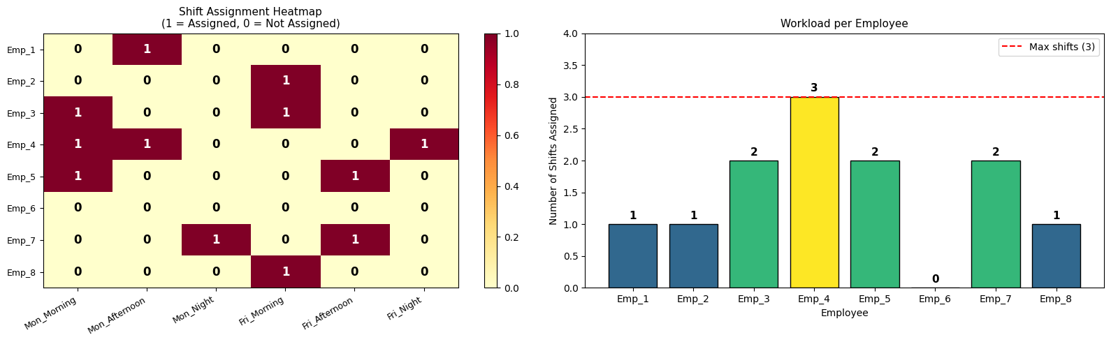
Chart 1 — Heatmap shows which employee is assigned to which shift. Yellow = unassigned, orange/red = assigned. Cell text is 0 or 1. Alongside it, a bar chart shows each employee’s workload compared to the maximum allowed.

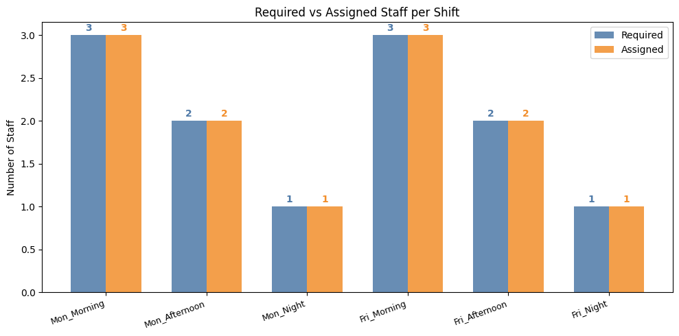
Chart 2 — Required vs Assigned Bar Chart compares how many staff were required vs actually assigned per shift. This quickly reveals if any shift is overstaffed (common since we minimize cost and constraints only require a minimum).

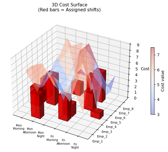
Chart 3 — 3D Cost Surface renders the full cost matrix as a semi-transparent surface. Red 3D bars mark the actual assigned (employee, shift) pairs, making it easy to see whether the solver picked low-cost assignments from the cost landscape.


Execution Results

1
2
3
4
5
6
7
8
9
10
11
12
13
14
15
16
17
18
19
20
21
Status      : Optimal
Total Cost : 37

Employee Mon_Morning Mon_Afternoon Mon_Night Fri_Morning Fri_Afternoon Fri_Night
--------------------------------------------------------------------------------------------------------------------
Emp_1 . ✓ . . . . (total=1)
Emp_2 . . . ✓ . . (total=1)
Emp_3 ✓ . . ✓ . . (total=2)
Emp_4 ✓ ✓ . . . ✓ (total=3)
Emp_5 ✓ . . . ✓ . (total=2)
Emp_6 . . . . . . (total=0)
Emp_7 . . ✓ . ✓ . (total=2)
Emp_8 . . . ✓ . . (total=1)

Staffing per shift:
Mon_Morning : assigned=3, required=3 [OK]
Mon_Afternoon : assigned=2, required=2 [OK]
Mon_Night : assigned=1, required=1 [OK]
Fri_Morning : assigned=3, required=3 [OK]
Fri_Afternoon : assigned=2, required=2 [OK]
Fri_Night : assigned=1, required=1 [OK]


All visualizations complete.

Key Takeaways

The ILP approach guarantees a globally optimal solution — no heuristic approximation. PuLP with CBC handles this small problem (8×6 binary variables) in milliseconds. For larger problems (hundreds of employees, 30-day scheduling horizons), the same model structure remains valid; you would simply swap CBC for a commercial solver like Gurobi or CPLEX, or apply decomposition techniques like column generation to keep solve times tractable.

The cost matrix can encode rich real-world preferences: overtime costs $c_{ij}^{OT}$, skill-mismatch penalties $c_{ij}^{skill}$, or employee preferences $c_{ij}^{pref}$, all summed into a single composite cost per assignment. This flexibility is one of the main reasons ILP remains the standard approach for real-world workforce scheduling.