Solving with Python
What is the 0-1 Capital Investment Selection Problem?
The 0-1 Capital Investment Selection Problem is a classic combinatorial optimization problem where a company must decide which investment projects to undertake given a limited budget. Each project is either selected (1) or not selected (0) — you can’t partially invest.
This is a variant of the 0-1 Knapsack Problem, and can be formulated as:
$$\max \sum_{i=1}^{n} v_i x_i$$
Subject to:
$$\sum_{i=1}^{n} c_i x_i \leq B$$
$$x_i \in {0, 1}, \quad i = 1, 2, \ldots, n$$
Where:
- $v_i$ = expected NPV (Net Present Value) of project $i$
- $c_i$ = required investment cost of project $i$
- $B$ = total available budget
- $x_i$ = binary decision variable (1 = invest, 0 = skip)
Concrete Example
A company has a budget of ¥500 million and is evaluating 10 candidate projects:
| Project | Cost (¥M) | Expected NPV (¥M) |
|---|---|---|
| P1 | 120 | 150 |
| P2 | 80 | 100 |
| P3 | 200 | 230 |
| P4 | 150 | 160 |
| P5 | 60 | 90 |
| P6 | 170 | 200 |
| P7 | 90 | 110 |
| P8 | 50 | 70 |
| P9 | 130 | 140 |
| P10 | 40 | 65 |
Goal: Maximize total NPV within the ¥500M budget.
Python Code
1 | # ============================================================ |
Code Walkthrough
Section 1 — Problem Data
Ten projects are defined with their respective costs and expected NPVs. These are stored as NumPy arrays for efficient computation.
Section 2 — Dynamic Programming Solver
This is the core algorithm. The DP table is defined as:
$$dp[i][w] = \text{maximum NPV achievable using the first } i \text{ projects with budget } w$$
The recurrence relation is:
$$dp[i][w] = \begin{cases} dp[i-1][w] & \text{if } c_i > w \ \max(dp[i-1][w],; dp[i-1][w - c_i] + v_i) & \text{if } c_i \leq w \end{cases}$$
After filling the table, back-tracking reconstructs which projects were selected by tracing which transitions changed the DP value.
Time complexity: $O(n \cdot B)$, where $n=10$ and $B=500$, making it extremely fast.
Section 3 — Results
Selected projects, total cost, total NPV, and remaining budget are printed cleanly.
Section 4 — Profitability Index
The Profitability Index (PI) is calculated as:
$$PI_i = \frac{v_i}{c_i}$$
A high PI means more NPV per yen invested — useful for intuition, though greedy PI selection doesn’t guarantee optimality for this problem.
Section 5 — Visualizations
Six subplots are generated:
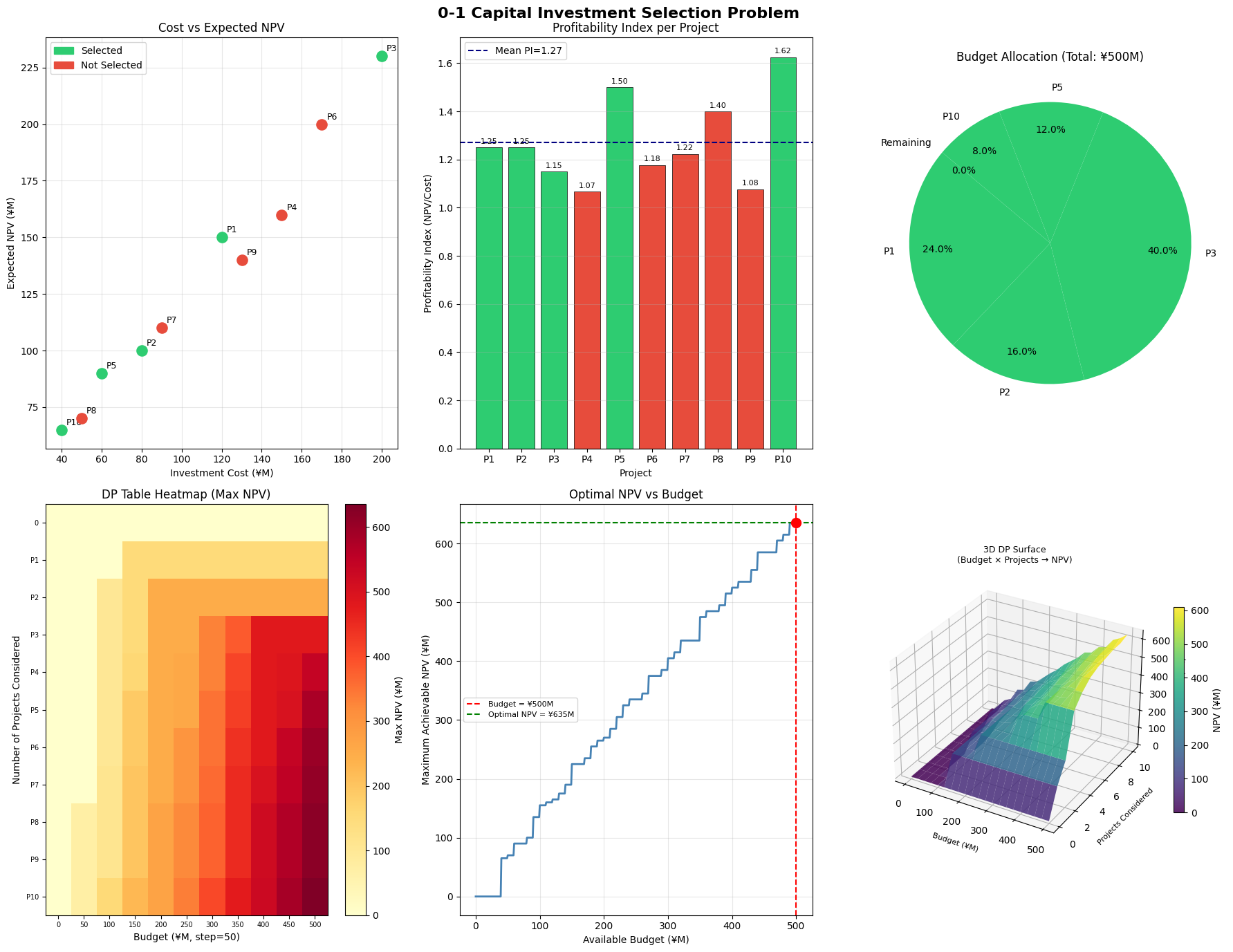
Plot 1 — Cost vs NPV Scatter: Shows each project as a dot. Green = selected, Red = not selected. Reveals which projects deliver high NPV relative to cost.
Plot 2 — Profitability Index Bar Chart: Ranks projects by NPV efficiency. The dashed line marks the average PI. Notably, a high PI doesn’t always mean a project gets selected — budget constraints may force trade-offs.
Plot 3 — Budget Allocation Pie Chart: Visualizes how the ¥500M budget is distributed among selected projects and remaining slack.
Plot 4 — DP Table Heatmap: Shows the full DP table as a 2D color map. The x-axis is the budget level (step=¥50M), and the y-axis is the number of projects considered. Darker colors = higher achievable NPV, clearly showing how value accumulates.
Plot 5 — Optimal NPV vs Budget Curve: Plots the maximum achievable NPV as a function of available budget. The curve rises steeply at first then flattens — this is the efficient frontier of capital allocation.
Plot 6 — 3D Surface Plot: The most visually powerful chart. It shows the entire DP surface:
- X-axis: budget
- Y-axis: number of projects considered
- Z-axis: maximum NPV
The surface illustrates how both budget and project count jointly determine the best achievable NPV, giving deep intuition into the optimization landscape.
Execution Results
=============================================
  0-1 Capital Investment Selection Result
=============================================
  Budget           : ¥500 M
  Selected Projects: ['P1', 'P2', 'P3', 'P5', 'P10']
  Total Cost       : ¥500 M
  Total NPV        : ¥635 M
  Remaining Budget : ¥0 M
=============================================
Graph saved as investment_selection.png
Key Takeaways
The DP approach guarantees the globally optimal solution — unlike greedy heuristics (e.g., always pick highest PI), it considers all valid combinations implicitly in $O(n \cdot B)$ time. For this problem:
$$\text{Optimal NPV} = \max \sum_{i \in S} v_i \quad \text{s.t.} \quad \sum_{i \in S} c_i \leq 500, \quad S \subseteq {1,\ldots,10}$$
This framework extends naturally to real-world capital budgeting scenarios with multiple budget periods, dependencies between projects, or risk-adjusted returns.