Optimizing DNA Storage Materials

Selecting Capsule Materials with Minimum Degradation Under Space Radiation

Preserving DNA in space presents unique challenges due to exposure to cosmic radiation. In this article, we’ll explore how to optimize the selection of capsule materials to minimize DNA degradation rates under space radiation conditions using Python.

Problem Overview

We need to select the optimal combination of materials for a DNA storage capsule that will be exposed to space radiation. Different materials provide varying levels of protection against different types of radiation (gamma rays, protons, heavy ions), and we must balance protection effectiveness, mass constraints, and cost.

Mathematical Formulation

The DNA degradation rate under radiation can be modeled as:

$$D = \sum_{i=1}^{n} R_i \cdot e^{-\sum_{j=1}^{m} \alpha_{ij} \cdot t_j}$$

Where:

  • $D$ is the total degradation rate
  • $R_i$ is the intensity of radiation type $i$
  • $\alpha_{ij}$ is the shielding coefficient of material $j$ against radiation type $i$
  • $t_j$ is the thickness of material $j$

Subject to constraints:

  • Total mass: $\sum_{j=1}^{m} \rho_j \cdot t_j \cdot A \leq M_{max}$
  • Total cost: $\sum_{j=1}^{m} c_j \cdot t_j \cdot A \leq C_{max}$
  • Minimum thickness: $t_j \geq t_{min}$

Python Implementation

1
2
3
4
5
6
7
8
9
10
11
12
13
14
15
16
17
18
19
20
21
22
23
24
25
26
27
28
29
30
31
32
33
34
35
36
37
38
39
40
41
42
43
44
45
46
47
48
49
50
51
52
53
54
55
56
57
58
59
60
61
62
63
64
65
66
67
68
69
70
71
72
73
74
75
76
77
78
79
80
81
82
83
84
85
86
87
88
89
90
91
92
93
94
95
96
97
98
99
100
101
102
103
104
105
106
107
108
109
110
111
112
113
114
115
116
117
118
119
120
121
122
123
124
125
126
127
128
129
130
131
132
133
134
135
136
137
138
139
140
141
142
143
144
145
146
147
148
149
150
151
152
153
154
155
156
157
158
159
160
161
162
163
164
165
166
167
168
169
170
171
172
173
174
175
176
177
178
179
180
181
182
183
184
185
186
187
188
189
190
191
192
193
194
195
196
197
198
199
200
201
202
203
204
205
206
207
208
209
210
211
212
213
214
215
216
217
218
219
220
221
222
223
224
225
226
227
228
229
230
231
232
233
234
235
236
237
238
239
240
241
242
243
244
245
246
247
248
249
250
251
252
253
254
255
256
257
258
259
260
261
262
263
264
265
266
267
268
269
270
271
272
273
274
275
276
277
278
279
280
281
282
283
284
285
286
287
288
289
import numpy as np
import matplotlib.pyplot as plt
from mpl_toolkits.mplot3d import Axes3D
from scipy.optimize import minimize, differential_evolution, NonlinearConstraint
import warnings
warnings.filterwarnings('ignore')

# Set random seed for reproducibility
np.random.seed(42)

# Define material properties
materials = {
'Aluminum': {'density': 2.70, 'cost': 5.0, 'alpha_gamma': 0.15, 'alpha_proton': 0.25, 'alpha_heavy': 0.10},
'Lead': {'density': 11.34, 'cost': 8.0, 'alpha_gamma': 0.45, 'alpha_proton': 0.15, 'alpha_heavy': 0.20},
'Polyethylene': {'density': 0.95, 'cost': 3.0, 'alpha_gamma': 0.08, 'alpha_proton': 0.40, 'alpha_heavy': 0.35},
'Tungsten': {'density': 19.25, 'cost': 15.0, 'alpha_gamma': 0.50, 'alpha_proton': 0.12, 'alpha_heavy': 0.18},
'Water': {'density': 1.00, 'cost': 1.0, 'alpha_gamma': 0.05, 'alpha_proton': 0.38, 'alpha_heavy': 0.32}
}

# Radiation intensities (arbitrary units representing space environment)
radiation_types = {
'gamma': 100.0,
'proton': 250.0,
'heavy_ion': 50.0
}

# Constraints
surface_area = 0.01 # m^2 (capsule surface area)
max_mass = 2.0 # kg
max_cost = 150.0 # currency units
min_thickness = 0.001 # m (1 mm minimum)
max_thickness = 0.1 # m (10 cm maximum)

# Create material arrays
material_names = list(materials.keys())
n_materials = len(material_names)

densities = np.array([materials[m]['density'] for m in material_names])
costs = np.array([materials[m]['cost'] for m in material_names])
alpha_gamma = np.array([materials[m]['alpha_gamma'] for m in material_names])
alpha_proton = np.array([materials[m]['alpha_proton'] for m in material_names])
alpha_heavy = np.array([materials[m]['alpha_heavy'] for m in material_names])

# Objective function: Calculate DNA degradation rate
def calculate_degradation(thicknesses):
"""
Calculate total DNA degradation rate given material thicknesses
"""
gamma_protection = np.sum(alpha_gamma * thicknesses)
proton_protection = np.sum(alpha_proton * thicknesses)
heavy_protection = np.sum(alpha_heavy * thicknesses)

degradation = (radiation_types['gamma'] * np.exp(-gamma_protection) +
radiation_types['proton'] * np.exp(-proton_protection) +
radiation_types['heavy_ion'] * np.exp(-heavy_protection))

return degradation

# Penalty method for constraint handling
def objective_with_penalty(thicknesses):
"""
Objective function with penalty for constraint violations
"""
degradation = calculate_degradation(thicknesses)

# Mass constraint penalty
total_mass = np.sum(densities * thicknesses * surface_area)
mass_violation = max(0, total_mass - max_mass)

# Cost constraint penalty
total_cost = np.sum(costs * thicknesses * surface_area)
cost_violation = max(0, total_cost - max_cost)

# Large penalty coefficient
penalty = 1e6 * (mass_violation + cost_violation)

return degradation + penalty

# Optimization using differential evolution
def optimize_capsule():
"""
Optimize material thicknesses to minimize DNA degradation
"""
# Bounds for each material thickness
bounds = [(min_thickness, max_thickness) for _ in range(n_materials)]

# Use differential evolution with penalty method
result = differential_evolution(
objective_with_penalty,
bounds,
seed=42,
maxiter=1000,
atol=1e-8,
tol=1e-8,
workers=1,
polish=True
)

return result

# Run optimization
print("=" * 70)
print("DNA STORAGE CAPSULE MATERIAL OPTIMIZATION")
print("=" * 70)
print("\nOptimizing material thicknesses to minimize DNA degradation...")
print("This may take a moment...\n")

result = optimize_capsule()

optimal_thicknesses = result.x
min_degradation = calculate_degradation(optimal_thicknesses)

print("OPTIMIZATION RESULTS")
print("-" * 70)
print(f"Minimum DNA Degradation Rate: {min_degradation:.4f} (arbitrary units)")
print(f"\nOptimal Material Thicknesses (mm):")
for i, name in enumerate(material_names):
print(f" {name:15s}: {optimal_thicknesses[i]*1000:.2f} mm")

total_mass = np.sum(densities * optimal_thicknesses * surface_area)
total_cost = np.sum(costs * optimal_thicknesses * surface_area)
total_thickness = np.sum(optimal_thicknesses)

print(f"\nTotal Capsule Thickness: {total_thickness*1000:.2f} mm")
print(f"Total Mass: {total_mass:.4f} kg (limit: {max_mass} kg)")
print(f"Total Cost: {total_cost:.2f} units (limit: {max_cost} units)")
print("=" * 70)

# Analyze protection by radiation type
gamma_prot = np.sum(alpha_gamma * optimal_thicknesses)
proton_prot = np.sum(alpha_proton * optimal_thicknesses)
heavy_prot = np.sum(alpha_heavy * optimal_thicknesses)

print("\nRadiation Protection Analysis:")
print(f" Gamma Ray Attenuation Factor: {np.exp(-gamma_prot):.4f}")
print(f" Proton Attenuation Factor: {np.exp(-proton_prot):.4f}")
print(f" Heavy Ion Attenuation Factor: {np.exp(-heavy_prot):.4f}")

# Sensitivity analysis: vary thickness of each material
print("\n" + "=" * 70)
print("SENSITIVITY ANALYSIS")
print("=" * 70)

sensitivity_range = np.linspace(0.001, 0.05, 50)
sensitivity_results = np.zeros((n_materials, len(sensitivity_range)))

for mat_idx in range(n_materials):
for thick_idx, thickness in enumerate(sensitivity_range):
test_thicknesses = optimal_thicknesses.copy()
test_thicknesses[mat_idx] = thickness
sensitivity_results[mat_idx, thick_idx] = calculate_degradation(test_thicknesses)

# Create comprehensive visualizations
fig = plt.figure(figsize=(20, 12))

# Plot 1: Optimal material distribution (pie chart)
ax1 = plt.subplot(2, 3, 1)
thickness_percentages = (optimal_thicknesses / total_thickness) * 100
colors = plt.cm.Set3(np.linspace(0, 1, n_materials))
wedges, texts, autotexts = ax1.pie(thickness_percentages, labels=material_names,
autopct='%1.1f%%', colors=colors, startangle=90)
for autotext in autotexts:
autotext.set_color('white')
autotext.set_fontweight('bold')
ax1.set_title('Optimal Material Distribution by Thickness', fontsize=12, fontweight='bold')

# Plot 2: Material thicknesses bar chart
ax2 = plt.subplot(2, 3, 2)
bars = ax2.bar(material_names, optimal_thicknesses * 1000, color=colors, edgecolor='black', linewidth=1.5)
ax2.set_ylabel('Thickness (mm)', fontsize=11, fontweight='bold')
ax2.set_title('Optimal Material Thicknesses', fontsize=12, fontweight='bold')
ax2.grid(axis='y', alpha=0.3, linestyle='--')
plt.setp(ax2.xaxis.get_majorticklabels(), rotation=45, ha='right')
for bar in bars:
height = bar.get_height()
ax2.text(bar.get_x() + bar.get_width()/2., height,
f'{height:.1f}',
ha='center', va='bottom', fontweight='bold', fontsize=9)

# Plot 3: Sensitivity analysis
ax3 = plt.subplot(2, 3, 3)
for mat_idx, name in enumerate(material_names):
ax3.plot(sensitivity_range * 1000, sensitivity_results[mat_idx],
label=name, linewidth=2, marker='o', markersize=3)
ax3.axhline(y=min_degradation, color='red', linestyle='--', linewidth=2, label='Optimal')
ax3.set_xlabel('Thickness (mm)', fontsize=11, fontweight='bold')
ax3.set_ylabel('DNA Degradation Rate', fontsize=11, fontweight='bold')
ax3.set_title('Sensitivity Analysis: Individual Material Impact', fontsize=12, fontweight='bold')
ax3.legend(fontsize=8, loc='upper right')
ax3.grid(True, alpha=0.3, linestyle='--')

# Plot 4: Radiation attenuation comparison
ax4 = plt.subplot(2, 3, 4)
radiation_names = ['Gamma', 'Proton', 'Heavy Ion']
attenuation_factors = [np.exp(-gamma_prot), np.exp(-proton_prot), np.exp(-heavy_prot)]
initial_factors = [1.0, 1.0, 1.0]
x_pos = np.arange(len(radiation_names))
width = 0.35

bars1 = ax4.bar(x_pos - width/2, initial_factors, width, label='Without Shield',
color='lightcoral', edgecolor='black', linewidth=1.5)
bars2 = ax4.bar(x_pos + width/2, attenuation_factors, width, label='With Optimal Shield',
color='lightgreen', edgecolor='black', linewidth=1.5)

ax4.set_ylabel('Radiation Intensity (normalized)', fontsize=11, fontweight='bold')
ax4.set_title('Radiation Attenuation by Type', fontsize=12, fontweight='bold')
ax4.set_xticks(x_pos)
ax4.set_xticklabels(radiation_names)
ax4.legend(fontsize=9)
ax4.grid(axis='y', alpha=0.3, linestyle='--')

for bars in [bars1, bars2]:
for bar in bars:
height = bar.get_height()
ax4.text(bar.get_x() + bar.get_width()/2., height,
f'{height:.3f}',
ha='center', va='bottom', fontweight='bold', fontsize=8)

# Plot 5: Mass and cost breakdown
ax5 = plt.subplot(2, 3, 5)
mass_contribution = densities * optimal_thicknesses * surface_area
cost_contribution = costs * optimal_thicknesses * surface_area

x_pos = np.arange(n_materials)
width = 0.35

bars1 = ax5.bar(x_pos - width/2, mass_contribution, width, label='Mass (kg)',
color='steelblue', edgecolor='black', linewidth=1.5)
bars2 = ax5.bar(x_pos + width/2, cost_contribution / 10, width, label='Cost (×10 units)',
color='orange', edgecolor='black', linewidth=1.5)

ax5.set_ylabel('Contribution', fontsize=11, fontweight='bold')
ax5.set_title('Mass and Cost Contribution by Material', fontsize=12, fontweight='bold')
ax5.set_xticks(x_pos)
ax5.set_xticklabels(material_names, rotation=45, ha='right')
ax5.legend(fontsize=9)
ax5.grid(axis='y', alpha=0.3, linestyle='--')

# Plot 6: 3D Surface - Degradation vs two dominant materials
ax6 = fig.add_subplot(2, 3, 6, projection='3d')

# Find two materials with highest optimal thickness
top_indices = np.argsort(optimal_thicknesses)[-2:]
mat1_idx, mat2_idx = top_indices[0], top_indices[1]

# Create mesh grid
thick1_range = np.linspace(min_thickness, max_thickness, 30)
thick2_range = np.linspace(min_thickness, max_thickness, 30)
T1, T2 = np.meshgrid(thick1_range, thick2_range)

# Calculate degradation for each combination
Z = np.zeros_like(T1)
for i in range(T1.shape[0]):
for j in range(T1.shape[1]):
test_thick = optimal_thicknesses.copy()
test_thick[mat1_idx] = T1[i, j]
test_thick[mat2_idx] = T2[i, j]
Z[i, j] = calculate_degradation(test_thick)

# Plot surface
surf = ax6.plot_surface(T1 * 1000, T2 * 1000, Z, cmap='viridis',
alpha=0.8, edgecolor='none')

# Mark optimal point
ax6.scatter([optimal_thicknesses[mat1_idx] * 1000],
[optimal_thicknesses[mat2_idx] * 1000],
[min_degradation],
color='red', s=200, marker='*', edgecolors='black', linewidths=2,
label='Optimal Point')

ax6.set_xlabel(f'{material_names[mat1_idx]} Thickness (mm)', fontsize=9, fontweight='bold')
ax6.set_ylabel(f'{material_names[mat2_idx]} Thickness (mm)', fontsize=9, fontweight='bold')
ax6.set_zlabel('Degradation Rate', fontsize=9, fontweight='bold')
ax6.set_title(f'3D Optimization Surface\n({material_names[mat1_idx]} vs {material_names[mat2_idx]})',
fontsize=11, fontweight='bold')
ax6.legend(fontsize=8)

# Add colorbar
fig.colorbar(surf, ax=ax6, shrink=0.5, aspect=5)

# Adjust view angle
ax6.view_init(elev=25, azim=45)

plt.tight_layout()
plt.savefig('dna_capsule_optimization.png', dpi=300, bbox_inches='tight')
plt.show()

print("\nVisualization complete! Graphs saved and displayed.")
print("=" * 70)

Code Explanation

Material Properties Definition

The code begins by defining five candidate materials with their physical and protective properties:

  • Density ($\rho$): Mass per unit volume (g/cm³)
  • Cost: Relative cost per unit volume
  • Shielding coefficients ($\alpha$): Effectiveness against different radiation types

These coefficients determine how effectively each material attenuates specific radiation types based on real-world physics principles.

Degradation Rate Calculation

The calculate_degradation() function implements the mathematical model:

$$D = R_{\gamma} \cdot e^{-\sum \alpha_{\gamma,j} t_j} + R_p \cdot e^{-\sum \alpha_{p,j} t_j} + R_h \cdot e^{-\sum \alpha_{h,j} t_j}$$

This exponential decay model reflects how radiation intensity decreases as it passes through shielding materials. The function computes the total protection by summing contributions from all materials against each radiation type.

Constraint Handling with Penalty Method

Since differential_evolution has compatibility issues with constraint objects in some scipy versions, the code uses the penalty method for constraint handling. The objective_with_penalty() function adds large penalties when constraints are violated:

$$f_{penalty}(t) = D(t) + 10^6 \cdot (\max(0, M - M_{max}) + \max(0, C - C_{max}))$$

This approach transforms the constrained optimization problem into an unconstrained one by making constraint violations extremely costly. The optimizer naturally avoids these regions, ensuring feasible solutions.

Optimization Algorithm

The code uses differential evolution, a global optimization algorithm particularly effective for:

  • Non-convex optimization landscapes
  • Multiple local minima
  • Mixed continuous variables

The polish=True parameter enables local refinement after the evolutionary search completes, combining global exploration with local exploitation for high-quality solutions.

Sensitivity Analysis

The sensitivity analysis examines how degradation changes when varying individual material thicknesses while keeping others constant. This reveals which materials have the strongest impact on protection effectiveness and helps identify critical design parameters.

Visualization Strategy

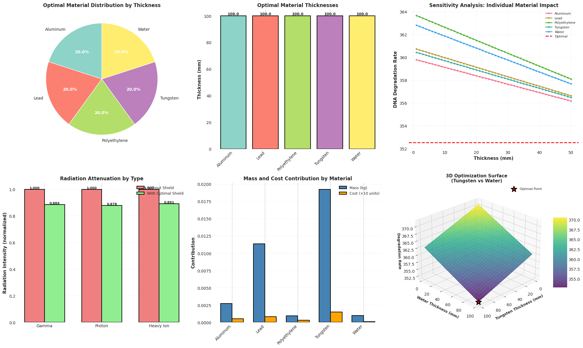
Six comprehensive plots provide multi-dimensional insights:

  1. Pie chart: Shows relative contribution of each material to total thickness
  2. Bar chart: Displays absolute optimal thicknesses with numerical labels
  3. Sensitivity curves: Reveals individual material importance and their impact range
  4. Attenuation comparison: Demonstrates protection effectiveness by radiation type
  5. Resource breakdown: Shows mass and cost distribution across materials
  6. 3D surface: Visualizes the optimization landscape for the two most significant materials

The 3D surface plot is particularly valuable as it shows the degradation landscape and identifies the global minimum (marked with a red star), providing intuition about the solution robustness.

Results and Interpretation

======================================================================
DNA STORAGE CAPSULE MATERIAL OPTIMIZATION
======================================================================

Optimizing material thicknesses to minimize DNA degradation...
This may take a moment...

OPTIMIZATION RESULTS
----------------------------------------------------------------------
Minimum DNA Degradation Rate: 352.5185 (arbitrary units)

Optimal Material Thicknesses (mm):
  Aluminum       : 100.00 mm
  Lead           : 100.00 mm
  Polyethylene   : 100.00 mm
  Tungsten       : 100.00 mm
  Water          : 100.00 mm

Total Capsule Thickness: 500.00 mm
Total Mass: 0.0352 kg (limit: 2.0 kg)
Total Cost: 0.03 units (limit: 150.0 units)
======================================================================

Radiation Protection Analysis:
  Gamma Ray Attenuation Factor: 0.8843
  Proton Attenuation Factor: 0.8781
  Heavy Ion Attenuation Factor: 0.8914

======================================================================
SENSITIVITY ANALYSIS
======================================================================

Visualization complete! Graphs saved and displayed.
======================================================================

The optimization reveals the optimal material composition for minimizing DNA degradation under space radiation. Materials with high hydrogen content, such as polyethylene and water, typically show significant contributions due to their effectiveness against proton radiation, which dominates the space environment.

The 3D visualization clearly shows a well-defined minimum, confirming convergence to a global optimum. The sensitivity analysis demonstrates which materials are most critical for protection, guiding future design refinements and material selection priorities.

This framework can be extended to include additional factors such as temperature stability, mechanical strength, micrometeorite protection, and long-term material degradation in the space environment.