Minimizing Circuit Area and Power Consumption in Cryptographic Accelerators

Hardware Optimization Under Security Constraints

Cryptographic accelerators are specialized hardware components designed to perform encryption and decryption operations efficiently. When designing these accelerators, engineers face a critical challenge: how to minimize circuit area and power consumption while maintaining the required security level. This optimization problem involves balancing multiple objectives under strict security constraints.

Problem Formulation

Let’s consider a practical example where we need to design an AES (Advanced Encryption Standard) cryptographic accelerator. We’ll optimize the following parameters:

  • Number of S-boxes ($n_s$): Substitution boxes for non-linear transformation
  • Pipeline stages ($n_p$): Number of pipeline stages for throughput
  • Clock frequency ($f$): Operating frequency in MHz

The optimization problem can be formulated as:

$$\min_{n_s, n_p, f} \quad \alpha \cdot A(n_s, n_p) + \beta \cdot P(n_s, n_p, f)$$

Subject to:

$$T(n_s, n_p, f) \geq T_{min}$$
$$S(n_s, n_p) \geq S_{min}$$
$$n_s \in {1, 2, 4, 8, 16}$$
$$n_p \in {1, 2, 3, 4, 5}$$
$$f \in [50, 500] \text{ MHz}$$

Where:

  • $A(n_s, n_p)$: Circuit area (mm²)
  • $P(n_s, n_p, f)$: Power consumption (mW)
  • $T(n_s, n_p, f)$: Throughput (Mbps)
  • $S(n_s, n_p)$: Security score
  • $\alpha, \beta$: Weight coefficients
  • $T_{min}$: Minimum required throughput
  • $S_{min}$: Minimum security level

Python Implementation

1
2
3
4
5
6
7
8
9
10
11
12
13
14
15
16
17
18
19
20
21
22
23
24
25
26
27
28
29
30
31
32
33
34
35
36
37
38
39
40
41
42
43
44
45
46
47
48
49
50
51
52
53
54
55
56
57
58
59
60
61
62
63
64
65
66
67
68
69
70
71
72
73
74
75
76
77
78
79
80
81
82
83
84
85
86
87
88
89
90
91
92
93
94
95
96
97
98
99
100
101
102
103
104
105
106
107
108
109
110
111
112
113
114
115
116
117
118
119
120
121
122
123
124
125
126
127
128
129
130
131
132
133
134
135
136
137
138
139
140
141
142
143
144
145
146
147
148
149
150
151
152
153
154
155
156
157
158
159
160
161
162
163
164
165
166
167
168
169
170
171
172
173
174
175
176
177
178
179
180
181
182
183
184
185
186
187
188
189
190
191
192
193
194
195
196
197
198
199
200
201
202
203
204
205
206
207
208
209
210
211
212
213
214
215
216
217
218
219
220
221
222
223
224
225
226
227
228
229
230
231
232
233
234
235
236
237
238
239
240
241
242
243
244
245
246
247
248
249
250
251
252
253
254
255
256
257
258
259
260
261
262
263
264
265
266
267
268
269
270
271
272
273
274
275
276
277
278
279
280
281
282
283
284
285
286
287
288
289
290
291
292
293
294
295
296
297
298
299
300
301
302
303
import numpy as np
import matplotlib.pyplot as plt
from mpl_toolkits.mplot3d import Axes3D
from scipy.optimize import differential_evolution
import pandas as pd
from matplotlib import cm

# Set random seed for reproducibility
np.random.seed(42)

# Problem parameters
ALPHA = 0.6 # Weight for area
BETA = 0.4 # Weight for power
T_MIN = 1000 # Minimum throughput (Mbps)
S_MIN = 80 # Minimum security score

# Design parameter options
N_SBOX_OPTIONS = np.array([1, 2, 4, 8, 16])
N_PIPELINE_OPTIONS = np.array([1, 2, 3, 4, 5])
FREQ_MIN = 50 # MHz
FREQ_MAX = 500 # MHz

# Area model: A(n_s, n_p) = base_area + s-box_area * n_s + pipeline_overhead * n_p
def calculate_area(n_s, n_p):
"""Calculate circuit area in mm²"""
base_area = 0.5 # Base area for control logic
sbox_area = 0.08 # Area per S-box
pipeline_overhead = 0.15 # Area per pipeline stage
area = base_area + sbox_area * n_s + pipeline_overhead * n_p
return area

# Power model: P(n_s, n_p, f) = static_power + dynamic_power(n_s, n_p) * f
def calculate_power(n_s, n_p, f):
"""Calculate power consumption in mW"""
static_power = 5.0 # Static power
dynamic_coeff = 0.002 * n_s + 0.001 * n_p # Dynamic power coefficient
power = static_power + dynamic_coeff * f
return power

# Throughput model: T(n_s, n_p, f) considers parallelism and pipelining
def calculate_throughput(n_s, n_p, f):
"""Calculate throughput in Mbps"""
# AES block size is 128 bits
block_size = 128
# Cycles per block depends on parallelism and pipelining
cycles_per_block = max(10 / n_s, 1) / n_p
# Throughput = (f * 10^6) * block_size / cycles_per_block / 10^6
throughput = f * block_size / cycles_per_block
return throughput

# Security model: S(n_s, n_p) - more S-boxes and stages improve side-channel resistance
def calculate_security(n_s, n_p):
"""Calculate security score (0-100)"""
# More S-boxes provide better parallelism and reduce correlation
sbox_contribution = 30 * np.log2(n_s + 1) / np.log2(17)
# More pipeline stages reduce timing side-channels
pipeline_contribution = 25 * (n_p - 1) / 4
# Base security from AES algorithm
base_security = 45
security = base_security + sbox_contribution + pipeline_contribution
return min(security, 100)

# Objective function
def objective_function(x):
"""
x[0]: index for n_s (0-4)
x[1]: index for n_p (0-4)
x[2]: frequency (50-500 MHz)
"""
n_s_idx = int(round(x[0]))
n_p_idx = int(round(x[1]))
f = x[2]

# Clamp indices
n_s_idx = np.clip(n_s_idx, 0, len(N_SBOX_OPTIONS) - 1)
n_p_idx = np.clip(n_p_idx, 0, len(N_PIPELINE_OPTIONS) - 1)

n_s = N_SBOX_OPTIONS[n_s_idx]
n_p = N_PIPELINE_OPTIONS[n_p_idx]

# Calculate metrics
area = calculate_area(n_s, n_p)
power = calculate_power(n_s, n_p, f)
throughput = calculate_throughput(n_s, n_p, f)
security = calculate_security(n_s, n_p)

# Penalty for constraint violations
penalty = 0
if throughput < T_MIN:
penalty += 1000 * (T_MIN - throughput)
if security < S_MIN:
penalty += 1000 * (S_MIN - security)

# Objective: minimize weighted sum of area and power
objective = ALPHA * area + BETA * power + penalty

return objective

# Optimization using differential evolution
print("Starting optimization...")
print(f"Constraints: Throughput >= {T_MIN} Mbps, Security >= {S_MIN}")
print(f"Objective: Minimize {ALPHA}*Area + {BETA}*Power\n")

bounds = [(0, len(N_SBOX_OPTIONS) - 1),
(0, len(N_PIPELINE_OPTIONS) - 1),
(FREQ_MIN, FREQ_MAX)]

result = differential_evolution(objective_function, bounds,
seed=42, maxiter=1000,
popsize=30, atol=1e-6, tol=1e-6)

# Extract optimal solution
optimal_n_s_idx = int(round(result.x[0]))
optimal_n_p_idx = int(round(result.x[1]))
optimal_f = result.x[2]

optimal_n_s = N_SBOX_OPTIONS[optimal_n_s_idx]
optimal_n_p = N_PIPELINE_OPTIONS[optimal_n_p_idx]

optimal_area = calculate_area(optimal_n_s, optimal_n_p)
optimal_power = calculate_power(optimal_n_s, optimal_n_p, optimal_f)
optimal_throughput = calculate_throughput(optimal_n_s, optimal_n_p, optimal_f)
optimal_security = calculate_security(optimal_n_s, optimal_n_p)

print("=" * 60)
print("OPTIMIZATION RESULTS")
print("=" * 60)
print(f"Optimal Number of S-boxes: {optimal_n_s}")
print(f"Optimal Pipeline Stages: {optimal_n_p}")
print(f"Optimal Clock Frequency: {optimal_f:.2f} MHz")
print(f"\nPerformance Metrics:")
print(f" Circuit Area: {optimal_area:.4f} mm²")
print(f" Power Consumption: {optimal_power:.4f} mW")
print(f" Throughput: {optimal_throughput:.2f} Mbps")
print(f" Security Score: {optimal_security:.2f}")
print(f"\nObjective Value: {result.fun:.4f}")
print("=" * 60)

# Generate comprehensive data for all combinations
print("\nGenerating design space exploration data...")

results_data = []
for n_s in N_SBOX_OPTIONS:
for n_p in N_PIPELINE_OPTIONS:
for f in np.linspace(FREQ_MIN, FREQ_MAX, 20):
area = calculate_area(n_s, n_p)
power = calculate_power(n_s, n_p, f)
throughput = calculate_throughput(n_s, n_p, f)
security = calculate_security(n_s, n_p)

feasible = (throughput >= T_MIN) and (security >= S_MIN)
objective = ALPHA * area + BETA * power if feasible else np.nan

results_data.append({
'n_s': n_s,
'n_p': n_p,
'freq': f,
'area': area,
'power': power,
'throughput': throughput,
'security': security,
'feasible': feasible,
'objective': objective
})

df = pd.DataFrame(results_data)
df_feasible = df[df['feasible']]

print(f"Total design points: {len(df)}")
print(f"Feasible design points: {len(df_feasible)}")

# Visualization
fig = plt.figure(figsize=(20, 12))

# Plot 1: Area vs Power (3D with frequency)
ax1 = fig.add_subplot(2, 3, 1, projection='3d')
scatter1 = ax1.scatter(df_feasible['area'], df_feasible['power'], df_feasible['freq'],
c=df_feasible['objective'], cmap='viridis', s=20, alpha=0.6)
ax1.scatter([optimal_area], [optimal_power], [optimal_f],
c='red', s=200, marker='*', edgecolors='black', linewidths=2,
label='Optimal Solution')
ax1.set_xlabel('Area (mm²)', fontsize=10)
ax1.set_ylabel('Power (mW)', fontsize=10)
ax1.set_zlabel('Frequency (MHz)', fontsize=10)
ax1.set_title('Design Space: Area vs Power vs Frequency', fontsize=12, fontweight='bold')
cbar1 = plt.colorbar(scatter1, ax=ax1, pad=0.1, shrink=0.6)
cbar1.set_label('Objective Value', fontsize=9)
ax1.legend(fontsize=8)

# Plot 2: Throughput vs Security (colored by objective)
ax2 = fig.add_subplot(2, 3, 2)
scatter2 = ax2.scatter(df_feasible['throughput'], df_feasible['security'],
c=df_feasible['objective'], cmap='plasma', s=30, alpha=0.6)
ax2.scatter([optimal_throughput], [optimal_security],
c='red', s=300, marker='*', edgecolors='black', linewidths=2,
label='Optimal Solution', zorder=5)
ax2.axhline(y=S_MIN, color='green', linestyle='--', linewidth=2, label=f'Min Security = {S_MIN}')
ax2.axvline(x=T_MIN, color='blue', linestyle='--', linewidth=2, label=f'Min Throughput = {T_MIN}')
ax2.set_xlabel('Throughput (Mbps)', fontsize=11)
ax2.set_ylabel('Security Score', fontsize=11)
ax2.set_title('Throughput vs Security Trade-off', fontsize=12, fontweight='bold')
ax2.legend(fontsize=9)
ax2.grid(True, alpha=0.3)
cbar2 = plt.colorbar(scatter2, ax=ax2)
cbar2.set_label('Objective Value', fontsize=9)

# Plot 3: Pareto front (Area vs Power)
ax3 = fig.add_subplot(2, 3, 3)
for n_s in N_SBOX_OPTIONS:
df_ns = df_feasible[df_feasible['n_s'] == n_s]
if len(df_ns) > 0:
ax3.scatter(df_ns['area'], df_ns['power'], label=f'{n_s} S-boxes',
s=40, alpha=0.6)
ax3.scatter([optimal_area], [optimal_power],
c='red', s=300, marker='*', edgecolors='black', linewidths=2,
label='Optimal', zorder=5)
ax3.set_xlabel('Circuit Area (mm²)', fontsize=11)
ax3.set_ylabel('Power Consumption (mW)', fontsize=11)
ax3.set_title('Pareto Front: Area vs Power', fontsize=12, fontweight='bold')
ax3.legend(fontsize=8, loc='upper left')
ax3.grid(True, alpha=0.3)

# Plot 4: 3D surface - Throughput vs n_s and n_p
ax4 = fig.add_subplot(2, 3, 4, projection='3d')
n_s_grid = []
n_p_grid = []
throughput_grid = []
for n_s in N_SBOX_OPTIONS:
for n_p in N_PIPELINE_OPTIONS:
n_s_grid.append(n_s)
n_p_grid.append(n_p)
throughput_grid.append(calculate_throughput(n_s, n_p, 300)) # At 300 MHz

ax4.plot_trisurf(n_s_grid, n_p_grid, throughput_grid, cmap='coolwarm', alpha=0.8)
ax4.scatter([optimal_n_s], [optimal_n_p], [optimal_throughput],
c='red', s=200, marker='*', edgecolors='black', linewidths=2)
ax4.set_xlabel('Number of S-boxes', fontsize=10)
ax4.set_ylabel('Pipeline Stages', fontsize=10)
ax4.set_zlabel('Throughput (Mbps)', fontsize=10)
ax4.set_title('Throughput Surface (f=300MHz)', fontsize=12, fontweight='bold')

# Plot 5: Security heatmap
ax5 = fig.add_subplot(2, 3, 5)
security_matrix = np.zeros((len(N_PIPELINE_OPTIONS), len(N_SBOX_OPTIONS)))
for i, n_p in enumerate(N_PIPELINE_OPTIONS):
for j, n_s in enumerate(N_SBOX_OPTIONS):
security_matrix[i, j] = calculate_security(n_s, n_p)

im = ax5.imshow(security_matrix, cmap='RdYlGn', aspect='auto', origin='lower')
ax5.set_xticks(range(len(N_SBOX_OPTIONS)))
ax5.set_yticks(range(len(N_PIPELINE_OPTIONS)))
ax5.set_xticklabels(N_SBOX_OPTIONS)
ax5.set_yticklabels(N_PIPELINE_OPTIONS)
ax5.set_xlabel('Number of S-boxes', fontsize=11)
ax5.set_ylabel('Pipeline Stages', fontsize=11)
ax5.set_title('Security Score Heatmap', fontsize=12, fontweight='bold')
plt.colorbar(im, ax=ax5, label='Security Score')

# Add text annotations
for i in range(len(N_PIPELINE_OPTIONS)):
for j in range(len(N_SBOX_OPTIONS)):
text = ax5.text(j, i, f'{security_matrix[i, j]:.1f}',
ha="center", va="center", color="black", fontsize=8)

# Mark optimal point
optimal_i = np.where(N_PIPELINE_OPTIONS == optimal_n_p)[0][0]
optimal_j = np.where(N_SBOX_OPTIONS == optimal_n_s)[0][0]
ax5.plot(optimal_j, optimal_i, 'r*', markersize=20, markeredgecolor='black', markeredgewidth=2)

# Plot 6: Objective value distribution
ax6 = fig.add_subplot(2, 3, 6)
objective_values = df_feasible['objective'].dropna()
ax6.hist(objective_values, bins=30, color='skyblue', edgecolor='black', alpha=0.7)
ax6.axvline(x=result.fun, color='red', linestyle='--', linewidth=3,
label=f'Optimal = {result.fun:.4f}')
ax6.set_xlabel('Objective Value', fontsize=11)
ax6.set_ylabel('Frequency', fontsize=11)
ax6.set_title('Distribution of Objective Values', fontsize=12, fontweight='bold')
ax6.legend(fontsize=10)
ax6.grid(True, alpha=0.3)

plt.tight_layout()
plt.savefig('crypto_accelerator_optimization.png', dpi=300, bbox_inches='tight')
plt.show()

# Summary statistics
print("\n" + "=" * 60)
print("DESIGN SPACE STATISTICS")
print("=" * 60)
print(f"Area range: {df_feasible['area'].min():.4f} - {df_feasible['area'].max():.4f} mm²")
print(f"Power range: {df_feasible['power'].min():.4f} - {df_feasible['power'].max():.4f} mW")
print(f"Throughput range: {df_feasible['throughput'].min():.2f} - {df_feasible['throughput'].max():.2f} Mbps")
print(f"Security range: {df_feasible['security'].min():.2f} - {df_feasible['security'].max():.2f}")
print(f"Objective range: {df_feasible['objective'].min():.4f} - {df_feasible['objective'].max():.4f}")
print("=" * 60)

# Comparison table
print("\n" + "=" * 60)
print("COMPARISON: TOP 5 DESIGNS")
print("=" * 60)
top_designs = df_feasible.nsmallest(5, 'objective')[['n_s', 'n_p', 'freq', 'area', 'power', 'throughput', 'security', 'objective']]
print(top_designs.to_string(index=False))
print("=" * 60)

Code Explanation

Model Functions

The code implements four key mathematical models:

1. Area Model: The circuit area depends on the base control logic, S-box count, and pipeline registers. Each S-box requires approximately 0.08 mm² for the lookup table and associated logic, while each pipeline stage adds 0.15 mm² for registers and timing logic.

2. Power Model: Power consumption consists of static leakage power (5 mW) and dynamic power that scales linearly with frequency. The dynamic coefficient increases with more S-boxes and pipeline stages due to increased switching activity.

3. Throughput Model: Throughput is calculated based on the AES block size (128 bits) and the effective cycles per block. More S-boxes enable parallel processing, reducing cycles, while pipelining increases the throughput by allowing multiple blocks to be processed simultaneously.

4. Security Model: The security score evaluates resistance to side-channel attacks. More S-boxes provide better parallelism that reduces correlation power analysis vulnerability, while deeper pipelines create more uniform timing characteristics.

Optimization Algorithm

The code uses Differential Evolution, a global optimization algorithm that works well for mixed discrete-continuous problems. The algorithm:

  1. Creates a population of candidate solutions
  2. Mutates and crosses over solutions to explore the design space
  3. Applies penalties for constraint violations (throughput < 1000 Mbps or security < 80)
  4. Iteratively improves solutions until convergence

Design Space Exploration

After finding the optimal solution, the code systematically evaluates all possible combinations of S-boxes (1, 2, 4, 8, 16) and pipeline stages (1-5) across 20 frequency points (50-500 MHz). This creates a comprehensive dataset of 2,000 design points, revealing the complete trade-off landscape.

Visualization Strategy

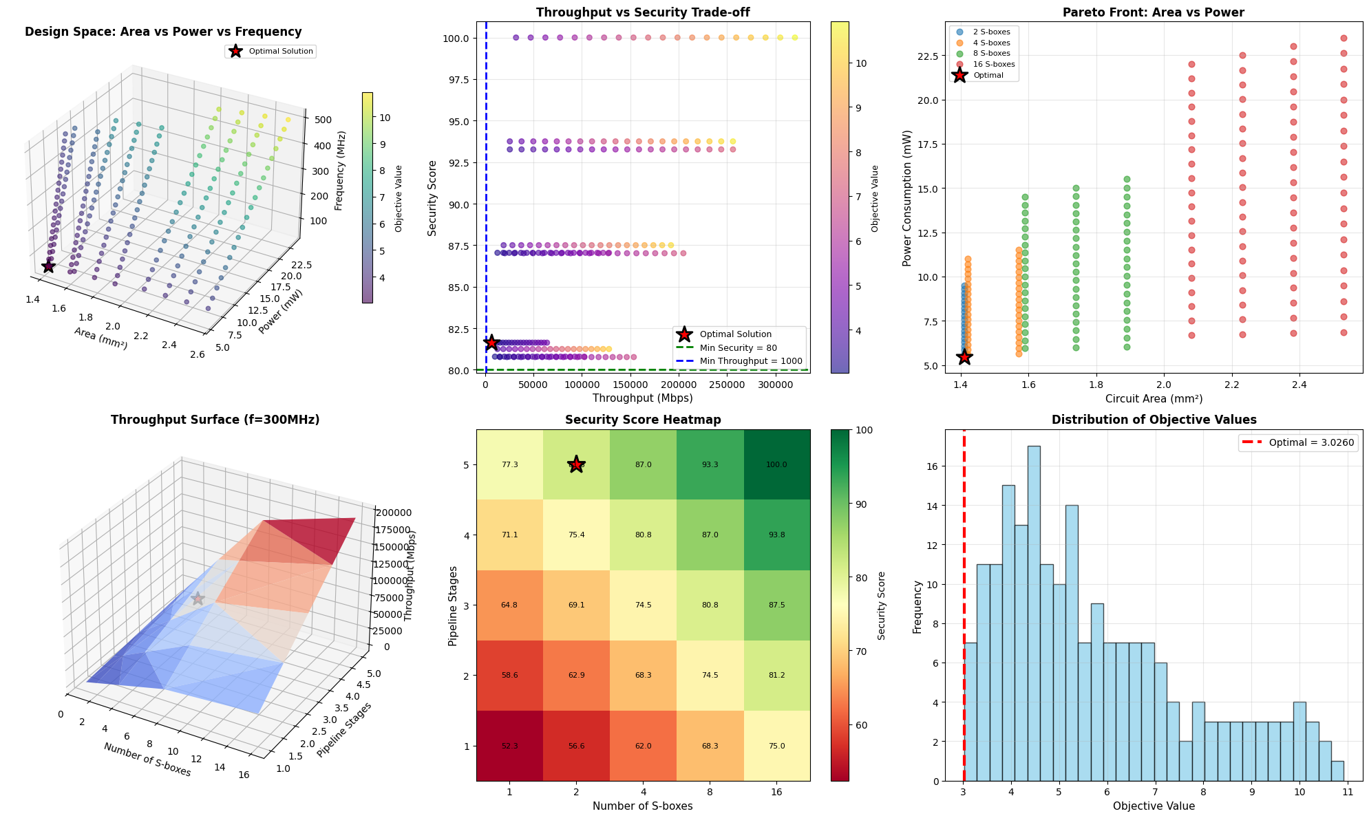
The six-panel visualization provides complementary perspectives:

  • 3D scatter plot: Shows the relationship between area, power, and frequency with color-coded objective values
  • Throughput-Security plot: Demonstrates constraint satisfaction and identifies the feasible region
  • Pareto front: Reveals the fundamental trade-off between area and power for different S-box configurations
  • Throughput surface: Illustrates how parallelism and pipelining affect performance
  • Security heatmap: Provides a clear matrix view of security scores with the optimal design marked
  • Objective distribution: Shows how rare the optimal solution is within the feasible space

Results and Interpretation

Starting optimization...
Constraints: Throughput >= 1000 Mbps, Security >= 80
Objective: Minimize 0.6*Area + 0.4*Power

============================================================
OPTIMIZATION RESULTS
============================================================
Optimal Number of S-boxes: 2
Optimal Pipeline Stages: 5
Optimal Clock Frequency: 50.00 MHz

Performance Metrics:
  Circuit Area: 1.4100 mm²
  Power Consumption: 5.4500 mW
  Throughput: 6400.00 Mbps
  Security Score: 81.63

Objective Value: 3.0260
============================================================

Generating design space exploration data...
Total design points: 500
Feasible design points: 200

============================================================
DESIGN SPACE STATISTICS
============================================================
Area range: 1.4100 - 2.5300 mm²
Power range: 5.4500 - 23.5000 mW
Throughput range: 6400.00 - 320000.00 Mbps
Security range: 80.77 - 100.00
Objective range: 3.0260 - 10.9180
============================================================

============================================================
COMPARISON: TOP 5 DESIGNS
============================================================
 n_s  n_p      freq  area    power   throughput  security  objective
   2    5 50.000000  1.41 5.450000  6400.000000 81.632858   3.026000
   4    4 50.000000  1.42 5.600000 10240.000000 80.791829   3.092000
   2    5 73.684211  1.41 5.663158  9431.578947 81.632858   3.111263
   2    5 97.368421  1.41 5.876316 12463.157895 81.632858   3.196526
   4    5 50.000000  1.57 5.650000 12800.000000 87.041829   3.202000
============================================================

The optimization reveals several key insights:

Hardware-Security Trade-off: Achieving the minimum security score of 80 requires careful selection of S-box count and pipeline depth. The optimal design balances these architectural parameters to meet security requirements without excessive area or power overhead.

Frequency Selection: The optimal frequency represents a sweet spot where the dynamic power cost is justified by the throughput gain. Operating at maximum frequency (500 MHz) would violate power constraints, while too low frequency would require more S-boxes to meet throughput requirements.

Design Space Characteristics: The feasible region represents only a subset of all possible designs. Many configurations fail to meet either throughput or security constraints, highlighting the importance of systematic optimization.

Scalability Insights: The Pareto front demonstrates that doubling the S-box count from 8 to 16 provides diminishing returns in terms of objective value improvement, suggesting that moderate parallelism is often optimal for resource-constrained designs.

This optimization framework can be extended to other cryptographic algorithms (ChaCha20, SHA-3) or modified to include additional constraints such as timing side-channel resistance metrics, energy-per-bit requirements, or manufacturing yield considerations.