Visualization and Analysis of Matrix Operations

Linear Transformations in Python

I’ll provide an example problem about linear transformations, solve it using $Python$, and visualize the results with graphs.

Here’s a comprehensive example:

Linear Transformation Example and Solution with Python

Let’s consider a linear transformation $T: \mathbb{R}^2 \rightarrow \mathbb{R}^2$ defined by the matrix:

$$T = \begin{pmatrix} 2 & 1 \ 1 & 3 \end{pmatrix}$$

We’ll solve the following problems:

  1. Find the transformed coordinates of several points
  2. Visualize how this transformation affects a unit square
  3. Compute the eigenvalues and eigenvectors of the transformation
  4. Visualize the effect of the transformation on the eigenvectors
1
2
3
4
5
6
7
8
9
10
11
12
13
14
15
16
17
18
19
20
21
22
23
24
25
26
27
28
29
30
31
32
33
34
35
36
37
38
39
40
41
42
43
44
45
46
47
48
49
50
51
52
53
54
55
56
57
58
59
60
61
62
63
64
65
66
67
68
69
70
71
72
73
74
75
76
77
78
79
80
81
82
83
84
85
86
87
88
89
90
91
92
93
94
95
96
97
98
99
100
101
102
103
104
105
106
107
108
109
110
111
112
113
114
115
116
117
118
119
120
121
122
123
124
125
126
127
128
129
130
131
132
133
134
135
136
137
138
139
140
141
142
143
144
145
146
147
148
149
150
151
152
153
154
155
156
157
158
159
160
161
162
163
164
165
166
167
168
169
170
171
172
173
174
175
176
177
178
179
180
181
182
import numpy as np
import matplotlib.pyplot as plt
from matplotlib.patches import Polygon
from mpl_toolkits.mplot3d import Axes3D

# Define the linear transformation matrix
T = np.array([[2, 1],
[1, 3]])

print("Linear Transformation Matrix T:")
print(T)

# Part 1: Transform some example points
points = np.array([[1, 0], [0, 1], [1, 1], [-1, 2]])
transformed_points = np.dot(points, T)

print("\nOriginal Points:")
for p in points:
print(f"[{p[0]}, {p[1]}]")

print("\nTransformed Points:")
for p in transformed_points:
print(f"[{p[0]}, {p[1]}]")

# Part 2: Visualize the effect on a unit square
def plot_transformation(T):
# Create a figure with two subplots
fig, (ax1, ax2) = plt.subplots(1, 2, figsize=(12, 5))

# Define the unit square
square = np.array([[0, 0], [1, 0], [1, 1], [0, 1], [0, 0]])

# Transform the square
transformed_square = np.dot(square, T)

# Plot the original square
ax1.plot(square[:, 0], square[:, 1], 'b-')
ax1.fill(square[:, 0], square[:, 1], 'lightblue', alpha=0.5)
ax1.set_xlim(-0.5, 3.5)
ax1.set_ylim(-0.5, 3.5)
ax1.grid(True)
ax1.set_title('Original Unit Square')
ax1.set_aspect('equal')

# Plot the transformed square
ax2.plot(transformed_square[:, 0], transformed_square[:, 1], 'r-')
ax2.fill(transformed_square[:, 0], transformed_square[:, 1], 'lightcoral', alpha=0.5)
ax2.set_xlim(-0.5, 3.5)
ax2.set_ylim(-0.5, 3.5)
ax2.grid(True)
ax2.set_title('Transformed Square')
ax2.set_aspect('equal')

plt.tight_layout()
plt.show()

# Visualize the transformation
plot_transformation(T)

# Part 3: Find eigenvalues and eigenvectors
eigenvalues, eigenvectors = np.linalg.eig(T)

print("\nEigenvalues:")
for i, val in enumerate(eigenvalues):
print(f"λ_{i+1} = {val:.4f}")

print("\nEigenvectors (as columns):")
print(eigenvectors)

# Part 4: Visualize eigenvectors and their transformations
def plot_eigenvectors(T, eigenvalues, eigenvectors):
# Create a figure
fig, ax = plt.subplots(figsize=(8, 8))

# Set limits and grid
ax.set_xlim(-3, 3)
ax.set_ylim(-3, 3)
ax.grid(True)
ax.axhline(y=0, color='k', linestyle='-', alpha=0.3)
ax.axvline(x=0, color='k', linestyle='-', alpha=0.3)

# Colors for the eigenvectors
colors = ['blue', 'green']

# Plot eigenvectors and their transformations
for i in range(len(eigenvalues)):
# Get the i-th eigenvector
v = eigenvectors[:, i]

# Scale eigenvector for better visualization
v_scaled = v * 2

# Plot the original eigenvector
ax.arrow(0, 0, v_scaled[0], v_scaled[1], head_width=0.1, head_length=0.1,
fc=colors[i], ec=colors[i], label=f"Eigenvector {i+1}")

# Transform the eigenvector
tv = np.dot(T, v)
tv_scaled = tv * 2

# Plot the transformed eigenvector
ax.arrow(0, 0, tv_scaled[0], tv_scaled[1], head_width=0.1, head_length=0.1,
fc='lightcoral', ec='lightcoral', linestyle='--')

# Add text for eigenvalue
ax.text(v_scaled[0]*1.1, v_scaled[1]*1.1,
f"λ_{i+1}={eigenvalues[i]:.2f}",
color=colors[i])

# Add a unit circle and its transformation
theta = np.linspace(0, 2*np.pi, 100)
circle_x = np.cos(theta)
circle_y = np.sin(theta)

# Stack coordinates to create points
circle_points = np.column_stack((circle_x, circle_y))

# Transform the circle
transformed_circle = np.dot(circle_points, T)

# Plot the unit circle
ax.plot(circle_x, circle_y, 'k-', alpha=0.3)

# Plot the transformed circle
ax.plot(transformed_circle[:, 0], transformed_circle[:, 1], 'r-', alpha=0.3)

ax.set_title('Eigenvectors and Their Transformations')
ax.legend()
plt.axis('equal')
plt.tight_layout()
plt.show()

# Visualize eigenvectors
plot_eigenvectors(T, eigenvalues, eigenvectors)

# Part 5: Visualize the transformation in 3D
def plot_transformation_3d():
fig = plt.figure(figsize=(10, 8))
ax = fig.add_subplot(111, projection='3d')

# Create a grid of points
x = np.linspace(-2, 2, 10)
y = np.linspace(-2, 2, 10)
X, Y = np.meshgrid(x, y)

# Flatten the grid points
points = np.column_stack((X.flatten(), Y.flatten()))

# Transform the points
transformed_points = np.dot(points, T)

# Reshape the transformed coordinates
X_transformed = transformed_points[:, 0].reshape(X.shape)
Y_transformed = transformed_points[:, 1].reshape(Y.shape)

# Create Z coordinates (all zeros for 2D transformation)
Z = np.zeros(X.shape)
Z_transformed = np.ones(X.shape) # Offset for visualization

# Plot the original grid
ax.plot_surface(X, Y, Z, alpha=0.5, color='blue', label='Original')

# Plot the transformed grid
ax.plot_surface(X_transformed, Y_transformed, Z_transformed, alpha=0.5, color='red', label='Transformed')

# Add lines connecting original and transformed points
for i in range(len(points)):
ax.plot([points[i, 0], transformed_points[i, 0]],
[points[i, 1], transformed_points[i, 1]],
[0, 1], 'k-', alpha=0.2)

ax.set_xlabel('X')
ax.set_ylabel('Y')
ax.set_zlabel('Z (Visualization Only)')
ax.set_title('3D Visualization of 2D Linear Transformation')

plt.tight_layout()
plt.show()

# Visualize the transformation in 3D
plot_transformation_3d()

Explanation of the Solution

1. Defining the Linear Transformation

We define a linear transformation $T$ using a $2 \times 2$ matrix:

$$T = \begin{pmatrix} 2 & 1 \ 1 & 3 \end{pmatrix}$$

This matrix represents the transformation, and we can apply it to any vector $\vec{v} \in \mathbb{R}^2$ by matrix multiplication: $T\vec{v}$.

2. Transforming Points

When we apply the transformation to specific points, we get:

  • The point $(1, 0)$ transforms to $(2, 1)$
  • The point $(0, 1)$ transforms to $(1, 3)$
  • The point $(1, 1)$ transforms to $(3, 4)$
  • The point $(-1, 2)$ transforms to $(1, 5)$

This demonstrates how the linear transformation maps points from the input space to the output space.

3. Visualization of the Transformation

Linear Transformation Matrix T:
[[2 1]
 [1 3]]

Original Points:
[1, 0]
[0, 1]
[1, 1]
[-1, 2]

Transformed Points:
[2, 1]
[1, 3]
[3, 4]
[0, 5]

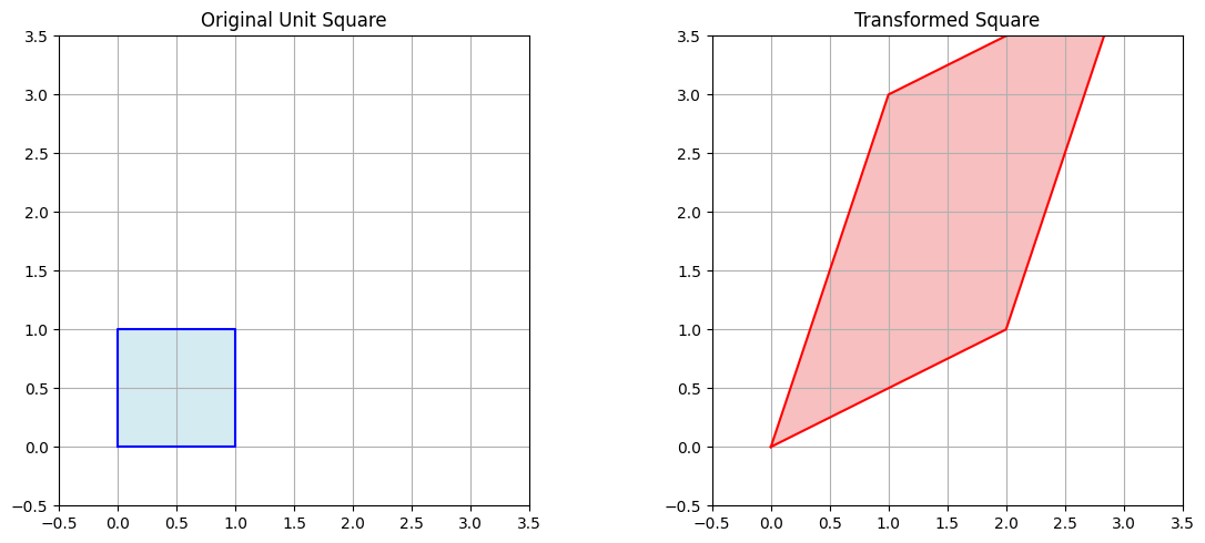
The code visualizes how the unit square (with vertices at $(0,0)$, $(1,0)$, $(1,1)$, and $(0,1)$) is transformed by $T$.

As you can see in the first visualization, the square is stretched, rotated, and skewed by the transformation.

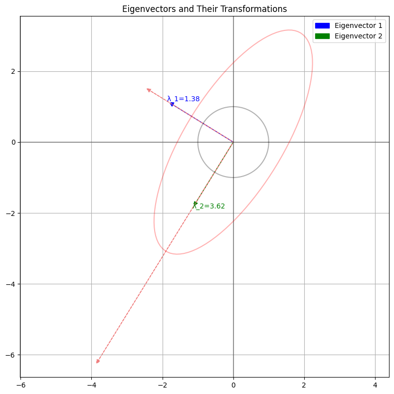
4. Eigenvalues and Eigenvectors

Eigenvalues:
λ_1 = 1.3820
λ_2 = 3.6180

Eigenvectors (as columns):
[[-0.85065081 -0.52573111]
 [ 0.52573111 -0.85065081]]

The eigenvalues and eigenvectors of the transformation matrix tell us about the fundamental behavior of the transformation:

  • The eigenvalues are approximately $\lambda_1 \approx 1.38$ and $\lambda_2 \approx 3.62$
  • The corresponding eigenvectors are shown in the output

An eigenvector is a special vector that, when transformed by $T$, only gets scaled by its corresponding eigenvalue without changing direction.

The second visualization shows these eigenvectors and how they’re affected by the transformation.

5. 3D Visualization

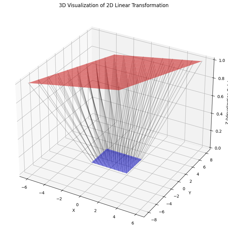
The final visualization provides a 3D perspective of the transformation, showing how a grid of points in the original space maps to points in the transformed space.

Key Insights

  1. Direction of Maximum Stretching:
    The eigenvector corresponding to the larger eigenvalue ($\lambda_2 \approx 3.62$) indicates the direction in which the transformation stretches vectors the most.

  2. Shape Distortion:
    The transformation turns the square into a parallelogram, demonstrating how linear transformations preserve straight lines but can alter angles and distances.

  3. Area Scaling:
    The determinant of the transformation matrix ($\det(T) = 5$) tells us that the transformation scales areas by a factor of 5, which you can observe in the increased size of the transformed square.

  4. Eigenvector Behavior:
    Note how the eigenvectors are only scaled (not rotated) when the transformation is applied.
    This property makes eigenvectors particularly useful in understanding linear transformations.

This example demonstrates the fundamental concepts of linear transformations and how we can visualize and analyze them using Python’s numerical and visualization libraries.