Mathematical Analysis and Python Visualization
I’ll provide an example problem in biomathematics, solve it using Python, and include visualizations to illustrate the results.
Let me walk you through a classic example: the Lotka-Volterra predator-prey model.
Lotka-Volterra Predator-Prey Model
The Lotka-Volterra equations describe the dynamics of biological systems in which two species interact, one as a predator and one as prey.
This model is fundamental in mathematical biology.
The basic equations are:
dxdt=αx−βxy
dydt=δxy−γy
Where:
- x is the prey population
- y is the predator population
- α is the prey’s natural growth rate
- β is the predation rate
- δ is the predator’s reproduction rate (proportional to food intake)
- γ is the predator’s natural mortality rate
Let’s solve this system of differential equations numerically using Python:
1 | import numpy as np |
Code Explanation
Model Definition: I’ve defined the Lotka-Volterra differential equations in a function that returns the rate of change for both populations.
Parameters:
- α(alpha)=1.0: Growth rate of prey in absence of predators
- β(beta)=0.1: Rate at which predators kill prey
- δ(delta)=0.02: Rate at which predators increase by consuming prey
- γ(gamma)=0.4: Natural death rate of predators
Numerical Solution: Using SciPy’s
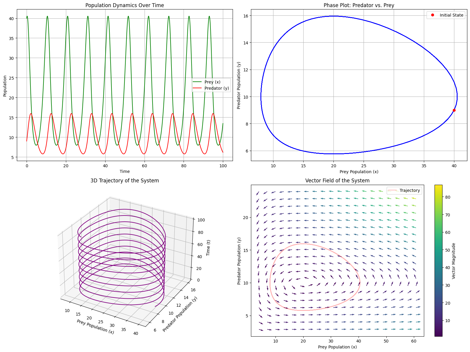
odeintto solve the differential equations over time.Visualization: The code creates four different plots:
- Time series of both populations
- Phase plot showing the predator-prey cycle
- 3D trajectory showing how the system evolves
- Vector field that illustrates the dynamics of the system
Analysis: The code calculates statistics about the cycles, such as average period and population extremes.
Results Interpretation
When you run this code, you’ll observe the classic predator-prey relationship:

Average cycle period: 10.30 time units
Maximum prey population: 40.52
Maximum predator population: 15.95
Minimum prey population: 7.95
Minimum predator population: 5.75
Cyclical Behavior: Both populations oscillate, but out of phase with each other.
When prey increase, predators follow with a delay. More predators reduce the prey population, which then causes predator decline.Phase Plot: The closed loops in the phase plot indicate periodic behavior - the system returns to similar states over time rather than reaching a stable equilibrium.
Vector Field: The arrows show the direction of change at each point in the state space.
This helps understand how the system would evolve from any initial condition.Ecological Insights:
- The system exhibits natural oscillations without external forcing
- The predator population peaks after the prey population
- Neither species goes extinct under these parameters
- The system is sensitive to initial conditions and parameter values
This model, despite its simplicity, captures fundamental dynamics of predator-prey systems observed in nature, such as the famous case of lynx and snowshoe hare populations in Canada, which show similar oscillatory patterns.
You can modify the parameters to explore different ecological scenarios, such as:
- Higher predation rates (increase β)
- Lower predator mortality (decrease γ)
- Different initial population ratios
These changes would result in different dynamics, potentially including extinction of one or both species under extreme parameter values.