Sorting Algorithm Performance

Problem Description

We will analyze the performance of three popular sorting algorithms:

  1. Bubble Sort (Simple but slow for large datasets),
  2. Merge Sort (Efficient divide-and-conquer algorithm),
  3. Python’s Built-in Timsort (Used by Python’s sorted() function).

The goal is to:

  1. Measure the time taken by each algorithm to sort a list of random numbers of increasing size.
  2. Visualize the time complexity and compare their performance.

Python Solution

1
2
3
4
5
6
7
8
9
10
11
12
13
14
15
16
17
18
19
20
21
22
23
24
25
26
27
28
29
30
31
32
33
34
35
36
37
38
39
40
41
42
43
44
45
46
47
48
49
50
51
52
53
54
55
56
57
58
59
60
61
62
63
64
65
66
67
68
69
70
71
72
73
74
75
76
77
78
79
80
81
82
83
84
85
86
87
88
89
90
import time
import random
import matplotlib.pyplot as plt

# Step 1: Implement sorting algorithms

# Bubble Sort
def bubble_sort(arr):
n = len(arr)
for i in range(n):
for j in range(0, n - i - 1):
if arr[j] > arr[j + 1]:
arr[j], arr[j + 1] = arr[j + 1], arr[j]

# Merge Sort
def merge_sort(arr):
if len(arr) > 1:
mid = len(arr) // 2
L = arr[:mid]
R = arr[mid:]

merge_sort(L)
merge_sort(R)

i = j = k = 0

while i < len(L) and j < len(R):
if L[i] < R[j]:
arr[k] = L[i]
i += 1
else:
arr[k] = R[j]
j += 1
k += 1

while i < len(L):
arr[k] = L[i]
i += 1
k += 1

while j < len(R):
arr[k] = R[j]
j += 1
k += 1

# Step 2: Test and time the algorithms
def test_sorting_algorithms():
sizes = [100, 500, 1000, 5000, 10000] # List sizes to test
bubble_times = []
merge_times = []
timsort_times = []

for size in sizes:
arr = [random.randint(0, 100000) for _ in range(size)]

# Bubble Sort
arr_copy = arr[:]
start_time = time.time()
bubble_sort(arr_copy)
bubble_times.append(time.time() - start_time)

# Merge Sort
arr_copy = arr[:]
start_time = time.time()
merge_sort(arr_copy)
merge_times.append(time.time() - start_time)

# Timsort (Python's built-in sorted())
arr_copy = arr[:]
start_time = time.time()
sorted(arr_copy)
timsort_times.append(time.time() - start_time)

return sizes, bubble_times, merge_times, timsort_times

# Step 3: Run the test
sizes, bubble_times, merge_times, timsort_times = test_sorting_algorithms()

# Step 4: Visualize the results
plt.figure(figsize=(10, 6))
plt.plot(sizes, bubble_times, label="Bubble Sort", marker='o', color='red')
plt.plot(sizes, merge_times, label="Merge Sort", marker='o', color='blue')
plt.plot(sizes, timsort_times, label="Timsort", marker='o', color='green')
plt.title("Sorting Algorithm Performance")
plt.xlabel("List Size")
plt.ylabel("Time Taken (seconds)")
plt.yscale("log") # Use logarithmic scale for better comparison
plt.grid(True, linestyle="--", alpha=0.6)
plt.legend()
plt.show()

Explanation of the Code

  1. Sorting Algorithms:

    • Bubble Sort:
      Compares adjacent elements and swaps them if they are in the wrong order.
      Very slow for large datasets $ O(n^2) $.
    • Merge Sort:
      Recursively divides the array into halves, sorts each half, and then merges them $ O(n \log n) $.
    • Timsort:
      Python’s optimized built-in algorithm, designed for real-world performance $ O(n \log n) $.
  2. Performance Measurement:

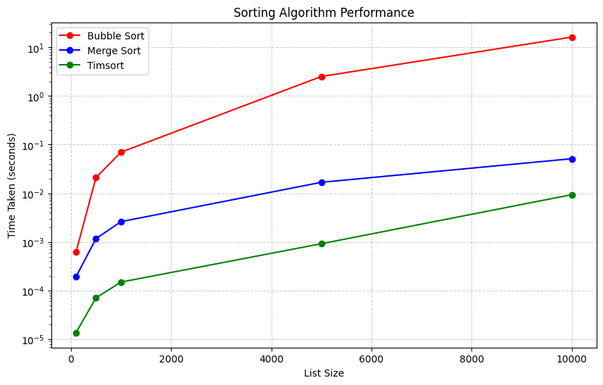
    • The algorithms are tested on arrays of increasing size: $100$, $500$, $1000$, $5000$, and $10,000$.
    • Execution time for each algorithm is measured using Python’s time module.
  3. Visualization:

    • The results are plotted with the list size on the $x$-axis and execution time on the $y$-axis.
    • A logarithmic scale is used for the $y$-axis to highlight differences between the algorithms.

Graph Explanation

  • X-axis:
    Represents the size of the list.
  • Y-axis:
    Represents the time taken (in seconds) on a logarithmic scale.
  • Observations:
    • Bubble Sort:
      The performance deteriorates rapidly as the list size increases, due to its quadratic time complexity $ O(n^2) $.
    • Merge Sort:
      Performs significantly better for large lists, maintaining $ O(n \log n) $ complexity.
    • Timsort:
      Outperforms both Bubble Sort and Merge Sort, as it is optimized for typical sorting use cases.

This example illustrates how algorithmic choices impact performance and the importance of selecting efficient algorithms for large datasets.