Problem Statement
A company produces a product whose profit P(x) (in dollars) as a function of production quantity x (in units) is modeled by the polynomial:
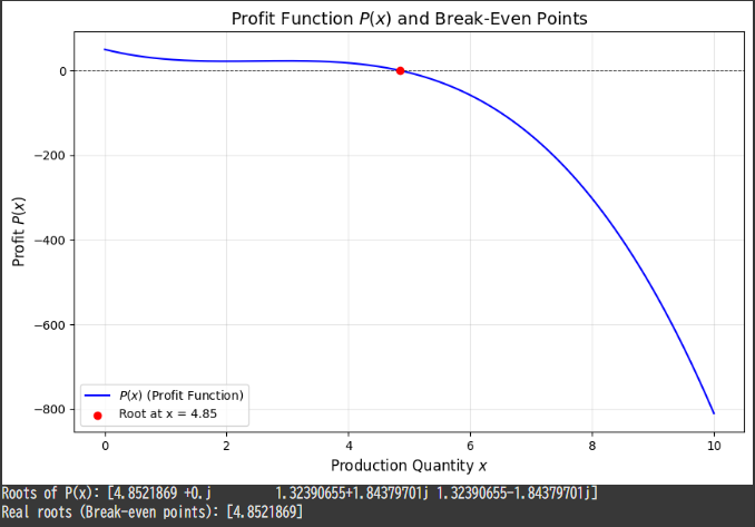
P(x)=−2x3+15x2−36x+50
- Determine the production quantities x (roots of P(x)=0) where the profit becomes zero (break-even points).
- Visualize the profit function P(x) to show its behavior and the identified roots.
Python Implementation
Here’s the Python code to solve the problem and visualize the results:
1 | import numpy as np |
Explanation of Code
Polynomial Representation:
- The profit function P(x)=−2x3+15x2−36x+50 is represented by its coefficients in decreasing powers of x.
- The
numpy.poly1dfunction creates a polynomial object for evaluation and visualization.
Root Finding:
- The roots of P(x) are found using
numpy.roots, which computes all roots (real and complex) of the polynomial. - Only real roots are relevant in this context as production quantities x must be real numbers.
- The roots of P(x) are found using
Visualization:
- The profit function is plotted over a reasonable range of x values (e.g., x∈[0,10]).
- Real roots (break-even points) are highlighted on the graph to show where the profit becomes zero.
Results and Graph Explanation

Numerical Results:
- Roots of P(x): These are the solutions to the equation P(x)=0.
Some may be complex, but only real roots are relevant for this real-world context. - Real roots (Break-even points): These are production levels where the company neither makes a profit nor a loss.
- Roots of P(x): These are the solutions to the equation P(x)=0.
Graph:
- The blue curve represents the profit function P(x).
- The red points indicate the break-even points where P(x)=0.
- The curve helps visualize how profit changes with production quantity x, showing regions of profit and loss.
By finding and plotting the roots of the polynomial, the company can identify critical production levels to optimize operations.