Least Squares and Regression with CVXPY
Least squares is a popular method for solving regression problems, where we want to fit a model to data by minimizing the sum of the squared differences (errors) between the observed values and the values predicted by the model.
In this example, we will demonstrate how to use CVXPY to solve a linear regression problem using least squares.
Problem Description: Linear Regression
We are given a dataset consisting of several observations.
Each observation includes:
- A set of features (independent variables).
- A target value (dependent variable).
Our goal is to find a linear relationship between the features and the target, meaning we want to find the best-fitting line (or hyperplane) that predicts the target based on the features.
Mathematically, we can express this as:
y=Xβ+ϵ
Where:
- (X) is a matrix of features (each row corresponds to an observation and each column to a feature).
- (y) is a vector of observed target values.
- (β) is the vector of unknown coefficients we want to estimate.
- (ϵ) represents the errors (differences between the predicted and observed values).
We want to find (β) that minimizes the sum of squared errors:
minβ|Xβ−y|22
Step-by-Step Solution with CVXPY
Here is how to solve this least squares problem using CVXPY:
1 | import numpy as np |
Detailed Explanation:
Data Generation:
In this example, we generate synthetic data for simplicity.
The matrix (X) contains 50 data points with 3 features, and we generate the target values (y) using a known set of coefficients (βtrue=[3,−1,2]) plus some noise to simulate real-world observations.Decision Variable:
The unknowns are the regression coefficients (β), represented as a CVXPY variablebetaof size 3 (since we have 3 features).Objective Function:
The goal is to minimize the sum of squared errors between the observed target values (y) and the predicted values (Xβ).
In CVXPY, this is represented by the functioncp.sum_squares(X @ beta - y), which computes the sum of the squared residuals.Problem Definition and Solution:
Thecp.Problemfunction defines the least squares optimization problem, andproblem.solve()finds the optimal solution for (β).Results:
After solving the problem, the estimated coefficients (β) are printed.
These should be close to the true coefficients used to generate the data.
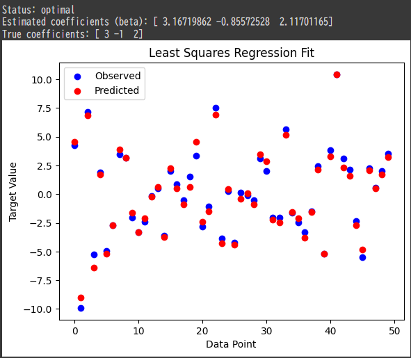
We also visualize the observed values versus the predicted values to show how well the model fits the data.
Output:
- Estimated Coefficients: The estimated coefficients (ˆβ) are close to the true coefficients used to generate the data ((βtrue=[3,−1,2])), which indicates a good fit.
Visualization of Results:
The following plot shows the observed values (in blue) and the predicted values (in red).
A good fit would show the predicted values closely following the observed ones.
- Blue points: Actual (observed) target values.
- Red points: Predicted target values based on the fitted model.
Interpretation:
Minimizing the Sum of Squared Errors:
The least squares method minimizes the squared differences between the predicted and observed values.
This produces the “best fit” line for the given data, in the sense that the total prediction error is minimized.Optimal Solution:
Since the status of the problem isoptimal, CVXPY successfully found the regression coefficients that minimize the objective function.
Conclusion:
In this example, we demonstrated how to solve a linear regression problem using least squares with CVXPY.
The least squares method is widely used in machine learning and statistics for fitting linear models to data.
By minimizing the sum of squared errors, we can estimate the coefficients that best explain the relationship between the features and the target values.

