線形最適化問題 CVXPY

線形最適化問題

CVXPYを使用して、簡単な線形最適化問題を解いてみましょう。

ここでは、2つの変数を持つ最小化の線形関数を扱います。例として、次のような問題を解いてみます。

$$
\text{minimize} \quad 3x + 4y
$$
$$
\text{subject to} \quad x + 2y \geq 10
$$
$$
\text{subject to} \quad 3x - y \leq 12
$$
$$
\text{subject to} \quad x, y \geq 0
$$

以下がそのコードです。

1
2
3
4
5
6
7
8
9
10
11
12
13
14
15
16
17
18
19
20
21
22
23
24
25
26
27
28
29
30
31
32
33
34
35
36
37
38
39
import cvxpy as cp
import numpy as np
import matplotlib.pyplot as plt

# 変数を定義
x = cp.Variable()
y = cp.Variable()

# 目的関数と制約条件を定義
objective = cp.Minimize(3*x + 4*y)
constraints = [x + 2*y >= 10, 3*x - y <= 12, x >= 0, y >= 0]

# 最適化問題の定義
problem = cp.Problem(objective, constraints)

# 問題を解く
problem.solve()

# 最適な解の表示
print("Optimal value:", problem.value)
print("x =", x.value)
print("y =", y.value)

# グラフ描画
x_values = np.linspace(0, 10, 100)
y1_values = (10 - x_values) / 2
y2_values = 3 * x_values - 12

plt.figure(figsize=(6, 6))
plt.plot(x_values, y1_values, label='x + 2y >= 10')
plt.plot(x_values, y2_values, label='3x - y <= 12')
plt.fill_between(x_values, np.maximum(0, y1_values), np.minimum(10, (12 + y2_values) / 3), color='gray', alpha=0.3)
plt.plot(x.value, y.value, 'ro') # 最適解のプロット
plt.xlabel('x')
plt.ylabel('y')
plt.title('Optimization with CVXPY')
plt.legend()
plt.grid(True)
plt.show()

これにより、線形最適化問題が解かれ、最適解が計算されます。

また、制約条件最適解が含まれたグラフも描画されます。

この場合、最適解は赤い点で示されます。

ソースコード解説

このコードは、CVXPYを使用して線形最適化問題を解決し、結果をグラフで視覚化するものです。

1. 必要なライブラリのインポート

1
2
3
import cvxpy as cp
import numpy as np
import matplotlib.pyplot as plt

必要なライブラリ(CVXPY、NumPy、Matplotlib)をインポートします。

2. 変数の定義

1
2
x = cp.Variable()
y = cp.Variable()

最適化問題で使用する変数 xy を定義しています。

3. 目的関数と制約条件の設定

1
2
objective = cp.Minimize(3*x + 4*y)
constraints = [x + 2*y >= 10, 3*x - y <= 12, x >= 0, y >= 0]

最小化したい目的関数制約条件を設定しています。

この場合、目的関数は$ (3x + 4y) $で、制約条件は不等式制約です。

4. 最適化問題の定義

1
problem = cp.Problem(objective, constraints)

CVXPYの Problem クラスを使って最適化問題を定義しています。

目的関数制約条件を引数として渡しています。

5. 問題の解決

1
problem.solve()

定義した最適化問題を解いています。
CVXPYが問題を解くための適切な最適化アルゴリズムを選択し、最適な解を見つけようとします。

6. 最適な解の表示

1
2
3
print("Optimal value:", problem.value)
print("x =", x.value)
print("y =", y.value)

最適な目的関数の値とそれに対する最適な変数 xy の値を表示しています。

7. グラフの描画

1
2
3
4
5
6
7
8
9
10
11
12
13
14
15
x_values = np.linspace(0, 10, 100)
y1_values = (10 - x_values) / 2
y2_values = 3 * x_values - 12

plt.figure(figsize=(6, 6))
plt.plot(x_values, y1_values, label='x + 2y >= 10')
plt.plot(x_values, y2_values, label='3x - y <= 12')
plt.fill_between(x_values, np.maximum(0, y1_values), np.minimum(10, (12 + y2_values) / 3), color='gray', alpha=0.3)
plt.plot(x.value, y.value, 'ro') # 最適解のプロット
plt.xlabel('x')
plt.ylabel('y')
plt.title('Optimization with CVXPY')
plt.legend()
plt.grid(True)
plt.show()

制約条件をグラフにプロットし、最適な解を赤い点として表示しています。

fill_between制約条件の領域を色で塗りつぶし、plt.plot最適解を赤い点でプロットしています。

結果解説

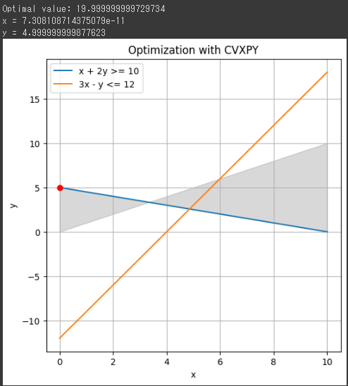
この結果は、与えられた線形最適化問題の最適な解を示しています。
最適な目的関数の値は約20です。

最適解は、$ (x \approx 0) $および$ (y \approx 5) $です。
つまり、制約条件を満たしながら最適な解が見つかりました。

グラフは、制約条件を表しています。
青い線はそれぞれ制約条件を示し、グレーの領域はすべての制約条件を満たす領域を示しています。
赤い点は最適解を表しており、制約条件の交差点に位置しています。
つまり、目的関数を最小化するための最適な$ (x) と (y) $の値を示しています。

最適解が$ (x \approx 0) $となる理由は、制約条件 $ (3x - y \leq 12) $により、$ (x) $が増加すると$ (y) $も増加する必要があるためです。
この条件を満たしつつ、目的関数を最小化するためには$ (x) $を極小化し$ (y) $を最大化するのが最適な戦略であり、その結果、$ (x \approx 0) $となります。