今回は、これまで実行してきたいろいろな分類モデルをまとめて評価します。
PR曲線の可視処理を関数化
まず、前回実行したPR曲線の可視化処理を関数化します。
[Google Colaboratory]
1 | def plot_pr_curve(y_true,proba): |
スケーリング
決定木以外のアルゴリズムのために、データのスケーリングを行います。
[Google Colaboratory]
1 | from sklearn.preprocessing import StandardScaler |
各モデルの定義
辞書型で各モデルの定義を行います。
[Google Colaboratory]
1 | from sklearn.linear_model import LogisticRegression |
SVCクラスでpredict_probaを使用するために、probabilityをTrueにします。
[Google Colaboratory]
1 | data_set = {"Train":[X_train_scaled,y_train],"Test":[X_test_scaled,y_test]} |
事前準備は以上で終了です。
各モデルの評価
各モデルごとに以下の処理を行います。
- モデルの構築・学習(4行目)
- 予測(11行目)
- データセットごとに分類レポートを出力(13~16行目)
output_dictをTrueにすることで辞書型で出力し、それをデータフレームにしています。 - テストデータに関してのPR曲線の可視化(20行目)
[Google Colaboratory]
1 | for model_name in models.keys(): |
各モデルの結果は次のようになりました。
[ロジスティック回帰の評価結果]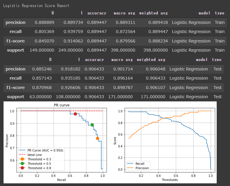
[線形SVMの評価結果]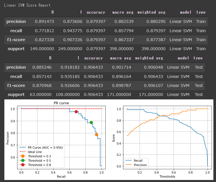
[カーネルSVMの評価結果]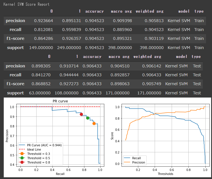
[K近傍法の評価結果]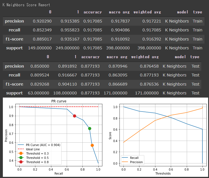
[決定木の評価結果]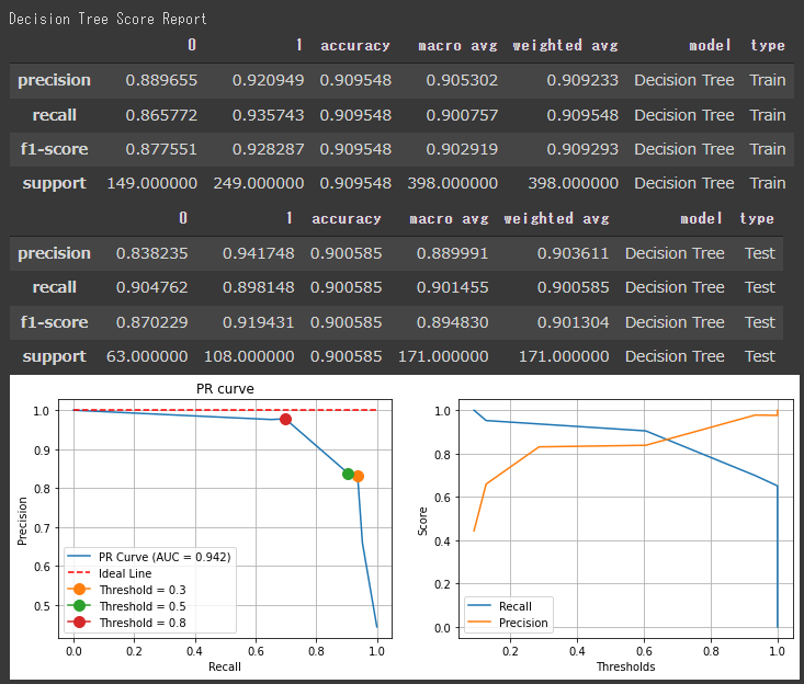
[ランダムフォレストの評価結果]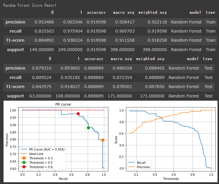
スコアを見ると、各アルゴリズムの評価に大きな差はないようです。
決定木やロジスティック回帰のF1値が高く出ているので、今回のデーセットに対しては、シンプルなアルゴリズムでもうまく分類できていると言えます。
分類レポートのスコアは全て閾値が50%として出力されているので、PR曲線などを見て閾値を調整すると評価結果が変わります。
いろいろな閾値を試してみると良いかもしれません。