価値反復法の1つQ学習で迷路を攻略します。
Q学習では1エピソードごとではなく1ステップごとに更新を行います。
まず使用するパッケージをインポートします。
1 | # 使用するパッケージの宣言 |
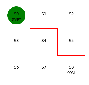
次に迷路の初期状態を描画します。
1 | # 初期位置での迷路の様子 |
初期の方策を決定するパラメータtheta_0を設定します。
行は状態0~7を表し、列は上、右、下、左へ行動できるかどうかを表します。
状態8はゴールなので方策の定義は不要です。
1 | # 初期の方策を決定するパラメータtheta_0を設定 |
方策パラメータθ0をランダム方策piに変換する関数を定義します。
1 | # 方策パラメータtheta_0をランダム方策piに変換する関数の定義 |
初期の行動価値関数Qを設定します。
行動価値関数は、行が状態sを表し、列が行動aを表します。
最初は正しい行動価値がわからないのでランダムな値を設定します。
1 | # 初期の行動価値関数Qを設定 |
ε-greedy法を実装します。
一定確率εでランダムに行動し、残りの1-εの確率で行動価値Qが最大になる行動をとります。
get_action()が行動を求める関数で、get_s_next()が行動を引数に次の状態を求める関数になります。
1 | # ε-greedy法を実装 |
行動価値関数Q(s,a)が正しい値になるように学習して更新する処理を実装します。
gammaは時間割引率で未来の報酬を割り引いています。
SarsaとQ学習の違いはこのコードだけになります。
Sarsaは更新時に次の行動を求めて更新に使用していましたが、Q学習では状態の行動価値関数の値のうち、最も大きいものを更新に使用します。
1 | # Q学習による行動価値関数Qの更新 |
Q学習に従って迷路を解く処理を実装します。
1 | # Q学習で迷路を解く関数の定義、状態と行動の履歴および更新したQを出力 |
価値関数の更新を繰り返す処理を実装します。
今回の学習終了条件は、100エピソードを行うこととしました。
Q学習で迷路を解く部分は、各エピソードでの状態価値関数の値を変数Vに格納しています。
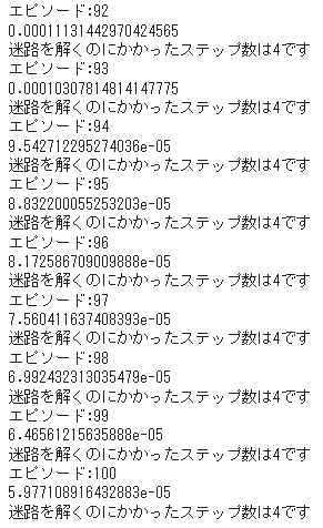
1 | # Q学習で迷路を解く |
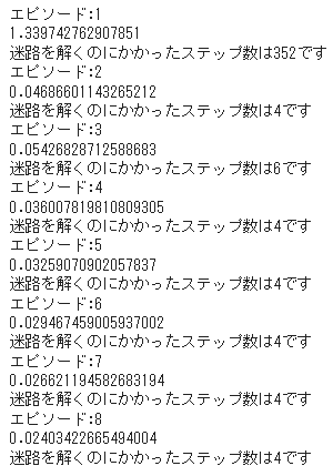
エピソード6以降はずっと最小の4ステップで安定しました。
エピソードごとに状態価値関数がどのように変化したのかを可視化します。
1 | # 状態価値の変化を可視化します |
最初は青だったマス目が次第に赤く変化していく様子が分かります。
完全に赤色にならないのは時間割引率で状態価値が割り引かれているためです。
ポイントは報酬が得られるゴールから逆向きに状態価値が学習されていくことと、学習後にはスタートからゴールへの道筋ができているということです。
(Google Colaboratoryで動作確認しています。)
参考
つくりながら学ぶ!深層強化学習 サポートページ