迷路を方策勾配法で解く

前回はランダムに行動する方策を実装しましたが、今回は方策勾配法に従ってエージェントを動かしてみます。

まず使用するパッケージをインポートします。

1
2
3
4
# 使用するパッケージの宣言
import numpy as np
import matplotlib.pyplot as plt
%matplotlib inline

次に迷路の初期状態を描画します。

1
2
3
4
5
6
7
8
9
10
11
12
13
14
15
16
17
18
19
20
21
22
23
24
25
26
27
28
29
30
31
32
# 初期位置での迷路の様子
# 図を描く大きさと、図の変数名を宣言
fig = plt.figure(figsize=(5, 5))
ax = plt.gca()

# 赤い壁を描く
plt.plot([1, 1], [0, 1], color='red', linewidth=2)
plt.plot([1, 2], [2, 2], color='red', linewidth=2)
plt.plot([2, 2], [2, 1], color='red', linewidth=2)
plt.plot([2, 3], [1, 1], color='red', linewidth=2)

# 状態を示す文字S0~S8を描く
plt.text(0.5, 2.5, 'S0', size=14, ha='center')
plt.text(1.5, 2.5, 'S1', size=14, ha='center')
plt.text(2.5, 2.5, 'S2', size=14, ha='center')
plt.text(0.5, 1.5, 'S3', size=14, ha='center')
plt.text(1.5, 1.5, 'S4', size=14, ha='center')
plt.text(2.5, 1.5, 'S5', size=14, ha='center')
plt.text(0.5, 0.5, 'S6', size=14, ha='center')
plt.text(1.5, 0.5, 'S7', size=14, ha='center')
plt.text(2.5, 0.5, 'S8', size=14, ha='center')
plt.text(0.5, 2.3, 'START', ha='center')
plt.text(2.5, 0.3, 'GOAL', ha='center')

# 描画範囲の設定と目盛りを消す設定
ax.set_xlim(0, 3)
ax.set_ylim(0, 3)
plt.tick_params(axis='both', which='both', bottom='off', top='off',
labelbottom='off', right='off', left='off', labelleft='off')

# 現在地S0に緑丸を描画する
line, = ax.plot([0.5], [2.5], marker="o", color='g', markersize=60)

実行結果1

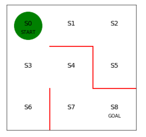
初期の方策を決定するパラメータtheta_0を設定します。

行は状態0~7を表し、列は上、右、下、左へ行動できるかどうかを表します。
状態8はゴールなので方策の定義は不要です。

1
2
3
4
5
6
7
8
9
10
11
# 初期の方策を決定するパラメータtheta_0を設定
# 行は状態0~7、列は移動方向で↑、→、↓、←を表す
theta_0 = np.array([[np.nan, 1, 1, np.nan], # s0
[np.nan, 1, np.nan, 1], # s1
[np.nan, np.nan, 1, 1], # s2
[1, 1, 1, np.nan], # s3
[np.nan, np.nan, 1, 1], # s4
[1, np.nan, np.nan, np.nan], # s5
[1, np.nan, np.nan, np.nan], # s6
[1, 1, np.nan, np.nan], # s7、※s8はゴールなので、方策はなし
])

方策パラメータ(theta)をsoftmax関数で行動方策(pi)に変換する関数を定義します。
betaは逆温度と呼ばれ、小さいほど行動がランダムになります。
さらに指数関数(np.exp)を使って割合を計算しています。

softmax関数を使用するとパラメータθが負の値になっても方策を算出できるというメリットがあります。

1
2
3
4
5
6
7
8
9
10
11
12
13
14
15
16
17
18
# 方策パラメータthetaを行動方策piにソフトマックス関数で変換する手法の定義
def softmax_convert_into_pi_from_theta(theta):
'''ソフトマックス関数で割合を計算する'''
beta = 1.0
[m, n] = theta.shape # thetaの行列サイズを取得
pi = np.zeros((m, n))

exp_theta = np.exp(beta * theta) # thetaをexp(theta)へと変換

for i in range(0, m):
# pi[i, :] = theta[i, :] / np.nansum(theta[i, :])
# simpleに割合の計算の場合
pi[i, :] = exp_theta[i, :] / np.nansum(exp_theta[i, :])
# softmaxで計算の場合

pi = np.nan_to_num(pi) # nanを0に変換

return pi

上記で定義したsoftmax_convert_into_pi_from_theta関数を使ってθ0から方策を算出します。

1
2
3
# 初期の方策pi_0を求める
pi_0 = softmax_convert_into_pi_from_theta(theta_0)
print(pi_0)

実行結果2
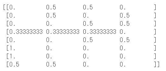
学習前のため前回(ランダム行動)の方策と同じ結果になりますが問題ありません。

続いてsoftmax関数による方策に従ってエージェントを行動させる関数を実装します。
1ステップ移動後のエージェントの状態とその時の行動を返します。

1
2
3
4
5
6
7
8
9
10
11
12
13
14
15
16
17
18
19
20
# 行動aと1step移動後の状態sを求める関数を定義
def get_action_and_next_s(pi, s):
direction = ["up", "right", "down", "left"]
# pi[s,:]の確率に従って、directionが選択される
next_direction = np.random.choice(direction, p=pi[s, :])

if next_direction == "up":
action = 0
s_next = s - 3 # 上に移動するときは状態の数字が3小さくなる
elif next_direction == "right":
action = 1
s_next = s + 1 # 右に移動するときは状態の数字が1大きくなる
elif next_direction == "down":
action = 2
s_next = s + 3 # 下に移動するときは状態の数字が3大きくなる
elif next_direction == "left":
action = 3
s_next = s - 1 # 左に移動するときは状態の数字が1小さくなる

return [action, s_next]

ゴールにたどり着くまでエージェントを移動させ続ける関数を定義します。
状態と行動の履歴をセットで返します。

1
2
3
4
5
6
7
8
9
10
11
12
13
14
15
16
17
18
19
# 迷路を解く関数の定義、状態と行動の履歴を出力
def goal_maze_ret_s_a(pi):
s = 0 # スタート地点
s_a_history = [[0, np.nan]] # エージェントの移動を記録するリスト

while (1): # ゴールするまでループ
[action, next_s] = get_action_and_next_s(pi, s)
s_a_history[-1][1] = action
# 現在の状態(つまり一番最後なのでindex=-1)の行動を代入

s_a_history.append([next_s, np.nan])
# 次の状態を代入。行動はまだ分からないのでnanにしておく

if next_s == 8: # ゴール地点なら終了
break
else:
s = next_s

return s_a_history

初期の方策で迷路を解いてみます。

1
2
3
4
# 初期の方策で迷路を解く
s_a_history = goal_maze_ret_s_a(pi_0)
print(s_a_history)
print("迷路を解くのにかかったステップ数は" + str(len(s_a_history) - 1) + "です")

実行結果3(途中略)
スタートからゴールまでの状態と行動のセットが表示されます。
最後にトータルで何ステップかかったかを表示しています。

方策勾配法に従い方策を更新する関数を定義します。

学習率etaは1回の学習で更新される大きさを表します。
学習率が小さすぎるとなかなか学習が進みませんし、大きすぎるときちんと学習することができません。

方策の更新のために下記の3つを入力しています。

  • 現在の方策 theta
  • 方策 pi
  • 現在の方策での実行結果 s_a_history
1
2
3
4
5
6
7
8
9
10
11
12
13
14
15
16
17
18
19
20
21
22
23
24
25
26
27
28
29
# thetaの更新関数を定義します
def update_theta(theta, pi, s_a_history):
eta = 0.1 # 学習率
T = len(s_a_history) - 1 # ゴールまでの総ステップ数

[m, n] = theta.shape # thetaの行列サイズを取得
delta_theta = theta.copy() # Δthetaの元を作成、ポインタ参照なので、delta_theta = thetaはダメ

# delta_thetaを要素ごとに求めます
for i in range(0, m):
for j in range(0, n):
if not(np.isnan(theta[i, j])): # thetaがnanでない場合

SA_i = [SA for SA in s_a_history if SA[0] == i]
# 履歴から状態iのものを取り出すリスト内包表記です

SA_ij = [SA for SA in s_a_history if SA == [i, j]]
# 状態iで行動jをしたものを取り出す

N_i = len(SA_i) # 状態iで行動した総回数
N_ij = len(SA_ij) # 状態iで行動jをとった回数

# 初版では符号の正負に間違いがありました(修正日:180703)
#delta_theta[i, j] = (N_ij + pi[i, j] * N_i) / T
delta_theta[i, j] = (N_ij - pi[i, j] * N_i) / T

new_theta = theta + eta * delta_theta

return new_theta

方策を更新し、方策がどう変化するのかを確認します。

1
2
3
4
# 方策の更新
new_theta = update_theta(theta_0, pi_0, s_a_history)
pi = softmax_convert_into_pi_from_theta(new_theta)
print(pi)

実行結果4
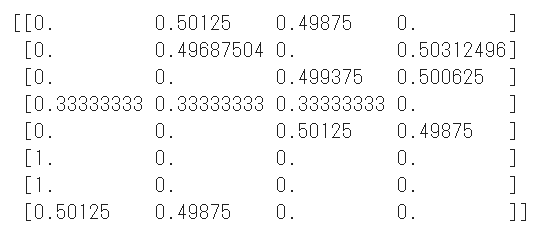
最初の方策から少し変化していることが分かります。

迷路をノーミスでクリアできるまで迷路内の探索とパラメータθの更新を繰り返す処理を実装します。

学習終了条件は課題に応じて調整する必要がありますが、今回は方策変化の絶対値和が10**-4より小さくなったら終了とします。

1
2
3
4
5
6
7
8
9
10
11
12
13
14
15
16
17
18
19
20
21
# 方策勾配法で迷路を解く
stop_epsilon = 10**-4 # 10^-4よりも方策に変化が少なくなったら学習終了とする

theta = theta_0
pi = pi_0

is_continue = True
count = 1
while is_continue: # is_continueがFalseになるまで繰り返す
s_a_history = goal_maze_ret_s_a(pi) # 方策πで迷路内を探索した履歴を求める
new_theta = update_theta(theta, pi, s_a_history) # パラメータΘを更新
new_pi = softmax_convert_into_pi_from_theta(new_theta) # 方策πの更新

print(np.sum(np.abs(new_pi - pi))) # 方策の変化を出力
print("迷路を解くのにかかったステップ数は" + str(len(s_a_history) - 1) + "です")

if np.sum(np.abs(new_pi - pi)) < stop_epsilon:
is_continue = False
else:
theta = new_theta
pi = new_pi

実行結果5(途中略)
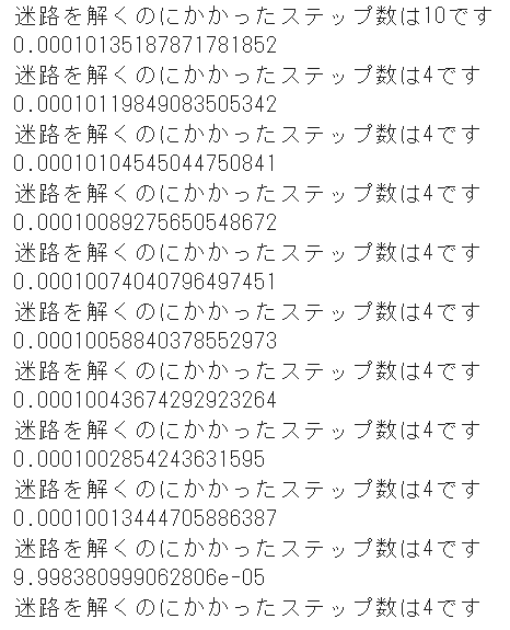
最終的にゴールまで最小ステップ数の4となっていることが分かります。
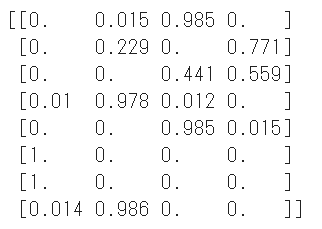
最終的な方策を確認してみます。

1
2
3
# 最終的な方策を確認
np.set_printoptions(precision=3, suppress=True) # 有効桁数3、指数表示しないという設定
print(pi)

実行結果6

最後に動画でエージェントの移動を可視化します。

1
2
3
4
5
6
7
8
9
10
11
12
13
14
15
16
17
18
19
20
21
22
23
# エージェントの移動の様子を可視化します
# 参考URL http://louistiao.me/posts/notebooks/embedding-matplotlib-animations-in-jupyter-notebooks/
from matplotlib import animation
from IPython.display import HTML

def init():
# 背景画像の初期化
line.set_data([], [])
return (line,)

def animate(i):
# フレームごとの描画内容
state = s_a_history[i][0] # 現在の場所を描く
x = (state % 3) + 0.5 # 状態のx座標は、3で割った余り+0.5
y = 2.5 - int(state / 3) # y座標は3で割った商を2.5から引く
line.set_data(x, y)
return (line,)

# 初期化関数とフレームごとの描画関数を用いて動画を作成
anim = animation.FuncAnimation(fig, animate, init_func=init, frames=len(
s_a_history), interval=500, repeat=False)

HTML(anim.to_jshtml())

スタート地点からまっすぐゴールにたどり着いていることが分かります。

(Google Colaboratoryで動作確認しています。)

参考

つくりながら学ぶ!深層強化学習 サポートページ