画像分類のためのニューラルネットワークを作成し、手書き数字の画像から数字を推論するモデルを作ります。
まず必要なパッケージをインポートします。
1 2 3 4 5 6 7 8 9 from tensorflow.keras.datasets import mnistfrom tensorflow.keras.layers import Activation, Dense, Dropoutfrom tensorflow.keras.models import Sequentialfrom tensorflow.keras.optimizers import SGDfrom tensorflow.keras.utils import to_categoricalimport numpy as npimport matplotlib.pyplot as plt%matplotlib inline
データセットの準備と確認を行います。
データセットの配列は下記のようになります。
配列
説明
train_images
訓練画像の配列
train_labels
訓練ラベルの配列
test_images
テスト画像の配列
test_labels
テストラベルの配列
データ型はNumpyのndarrayになります。この配列型を使うと高速な配列演算が可能になります。
1 2 (train_images, train_labels), (test_images, test_labels) = mnist.load_data()
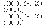
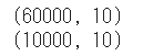
データセットのシェイプを確認します。
1 2 3 4 5 print (train_images.shape)print (train_labels.shape)print (test_images.shape)print (test_labels.shape)
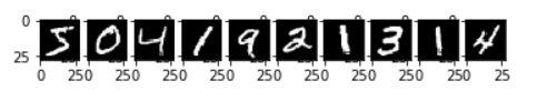
先頭10件の訓練画像を確認します。
1 2 3 4 5 for i in range (10 ): plt.subplot(1 , 10 , i+1 ) plt.imshow(train_images[i], 'gray' ) plt.show()
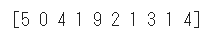
データセットのラベルを確認します。
実行結果3とラベルが合致していることが分かります。
1 2 print (train_labels[0 :10 ])
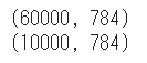
データセットをニューラルネットワークに適した形式に変換します。
2次元配列(28×28)を1次元配列(786)に変換します。
1 2 3 4 5 6 7 train_images = train_images.reshape((train_images.shape[0 ], 784 )) test_images = test_images.reshape((test_images.shape[0 ], 784 )) print (train_images.shape)print (test_images.shape)
訓練ラベルとテストラベルをone-hot表現に変換します。
one-hot表現とはある要素のみが1でそのほかの要素が0であるような表現です。
1 2 3 4 5 6 7 train_labels = to_categorical(train_labels) test_labels = to_categorical(test_labels) print (train_labels.shape)print (test_labels.shape)
ニューラルネットワークのモデルを作成します。
モデルのネットワーク構造は全結合層を3つ重ねたものです。
入力層が784(28×28)で出力層が10になります。
隠れ層は自由に決められますが今回は128としました。
過学習防止のためDropoutを設定します。
活性化関数はシグモイド関数とソフトマックス関数を使用します。
1 2 3 4 5 6 model = Sequential() model.add(Dense(256 , activation='sigmoid' , input_shape=(784 ,))) model.add(Dense(128 , activation='sigmoid' )) model.add(Dropout(rate=0.5 )) model.add(Dense(10 , activation='softmax' ))
ニューラルネットワークのモデルをコンパイルします。
コンパイル時には下記の3つを設定します。
損失関数
最適化関数
評価指標
1 2 model.compile (loss='categorical_crossentropy' , optimizer=SGD(lr=0.1 ), metrics=['acc' ])
訓練画像と訓練ラベルの配列をモデルに渡して学習を実行します。
1 2 3 history = model.fit(train_images, train_labels, batch_size=500 , epochs=5 , validation_split=0.2 )
学習時の結果(fit関数の戻り値)には次の情報が含まれています。
情報
説明
loss
訓練データの誤差。0に近いほどよい。
acc
訓練データの正解率。1に近いほどよい。
val_loss
検証データの誤差。0に近いほどよい。
val_acc
検証データの正解率。1に近いほどよい。
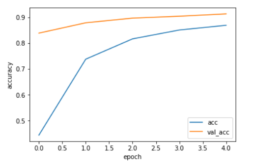
accとval_accをグラフ化してみます。
1 2 3 4 5 6 7 plt.plot(history.history['acc' ], label='acc' ) plt.plot(history.history['val_acc' ], label='val_acc' ) plt.ylabel('accuracy' ) plt.xlabel('epoch' ) plt.legend(loc='best' ) plt.show()
テスト画像とテストラベルの配列をモデルに渡して評価を行います。
1 2 3 test_loss, test_acc = model.evaluate(test_images, test_labels) print ('loss: {:.3f}\nacc: {:.3f}' .format (test_loss, test_acc ))
正解率が91%を超えていることが分かります。
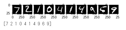
最後に先頭10件のテスト画像の推論を行い、予測結果を取得します、
1 2 3 4 5 6 7 8 9 10 for i in range (10 ): plt.subplot(1 , 10 , i+1 ) plt.imshow(test_images[i].reshape((28 , 28 )), 'gray' ) plt.show() test_predictions = model.predict(test_images[0 :10 ]) test_predictions = np.argmax(test_predictions, axis=1 ) print (test_predictions)
十分に正確な結果となっています。
(Google Colaboratory で動作確認しています。)
参考
AlphaZero 深層学習・強化学習・探索 人工知能プログラミング実践入門 サポートページ