Maximizing Gain and Controlling Directivity
Antenna design is fundamentally an optimization problem. Given constraints on physical size, operating frequency, and manufacturing tolerance, we want to find element configurations that maximize radiated power in desired directions while suppressing radiation elsewhere. This post works through a concrete phased-array example — optimizing complex excitation weights using both analytic gradient methods and metaheuristic search — and visualizes the results with 2D polar plots and a full 3D radiation pattern.
Problem Setup
Consider a uniform linear array (ULA) of $N$ isotropic radiating elements placed along the $z$-axis with inter-element spacing $d$. Element $n$ is located at $z_n = n \cdot d$, $n = 0, 1, \ldots, N-1$. Each element is driven by a complex weight $w_n = a_n e^{j\phi_n}$, where $a_n$ is the amplitude and $\phi_n$ is the phase.
The array factor in the elevation direction $\theta$ is:
$$AF(\theta) = \sum_{n=0}^{N-1} w_n , e^{j k n d \cos\theta}$$
where $k = 2\pi/\lambda$ is the free-space wavenumber and $\lambda$ is the wavelength. The normalized power pattern is:
$$P(\theta) = \frac{|AF(\theta)|^2}{\max_\theta |AF(\theta)|^2}$$
Directivity in the direction $\theta_0$ is:
$$D(\theta_0) = \frac{4\pi , |AF(\theta_0)|^2}{\displaystyle\int_0^{2\pi}\int_0^{\pi} |AF(\theta)|^2 \sin\theta , d\theta , d\phi}$$
For a ULA the $\phi$-integral is trivial (azimuthal symmetry), giving:
$$D(\theta_0) = \frac{2 , |AF(\theta_0)|^2}{\displaystyle\int_0^{\pi} |AF(\theta)|^2 \sin\theta , d\theta}$$
Gain $G = \eta \cdot D$, where $\eta$ is radiation efficiency; for lossless elements $G = D$.
Optimization Objective
We maximize directivity toward a steering angle $\theta_0 = 30°$ while constraining the side-lobe level (SLL) to be no worse than $-20$ dB relative to the main lobe:
$$\max_{\mathbf{w}} ; D(\theta_0), \qquad \text{subject to} \quad P(\theta) \leq 10^{-2} ; \forall , \theta \notin \Theta_{\text{main}}$$
where $\Theta_{\text{main}}$ is a $\pm 10°$ exclusion zone around $\theta_0$.
We solve this with two complementary approaches:
- Chebyshev / Dolph–Chebyshev taper — analytic closed-form that exactly achieves a prescribed SLL with minimum beam width.
- Differential Evolution (DE) — a global optimizer that directly maximizes directivity under an explicit SLL penalty, with no analytic structure assumed.
Full Source Code
1 | # ============================================================ |
Code Walkthrough
Section 0 — Global Parameters
1 | N = 16 |
All physical constants are declared once. k_d = 2π · d/λ absorbs both wavenumber and spacing. The steering vector matrix SV of shape (N_THETA, N) is precomputed once as:
$$SV_{i,n} = e^{j k d \cos\theta_i \cdot n}$$
so every subsequent pattern evaluation is a single matrix–vector multiply — the key performance trick.
Section 1 — Array Factor and Directivity
array_factor(weights) returns $|AF(\theta)|^2$ at all $N_{\theta}$ angles simultaneously via SV @ weights. directivity_at integrates the denominator with np.trapz over the $\sin\theta$ measure. sll_db_value masks out the $\pm\text{half_width}$ main-lobe exclusion zone before taking the peak.
Section 2 — Dolph–Chebyshev Taper
The Dolph–Chebyshev design maps the visible space $u \in [-1,1]$ to the argument of a Chebyshev polynomial of order $M = N-1$. The parameter:
$$x_0 = \cosh!\left(\frac{\cosh^{-1}R}{M}\right), \qquad R = 10^{-\text{SLL}/20}$$
stretches the Chebyshev equiripple region to exactly fill the side-lobe region. The IDFT trick evaluates the Chebyshev polynomial at $2N$ uniformly spaced points around the unit circle, then extracts the first $N$ IFFT coefficients as element amplitudes. This is $O(N \log N)$.
Progressive phase $\phi_n = -k d \cos\theta_0 \cdot n$ steers the beam to $\theta_0 = 30°$.
Section 3 — Differential Evolution
The decision vector $\mathbf{x} \in \mathbb{R}^{2N}$ packs amplitudes $a_n \in [0,1]$ and phases $\phi_n \in [-\pi, \pi]$. The objective is:
$$f(\mathbf{x}) = -D(\theta_0;\mathbf{w}) + 50 \cdot \max!\bigl(0,, \text{SLL}(\mathbf{w}) - \text{SLL}_{\text{target}}\bigr)$$
The penalty coefficient 50 is large enough to prevent SLL violations without overwhelming the directivity signal. scipy.optimize.differential_evolution with updating="deferred" evaluates the entire population before applying selection — more robust on multimodal landscapes. polish=True applies a local L-BFGS-B refinement on the best individual.
Sections 4–6 — Uniform Baseline and Visualisation
All three weight vectors are evaluated and compared on directivity and SLL. Five figures are produced:
| Figure | Content |
|---|---|
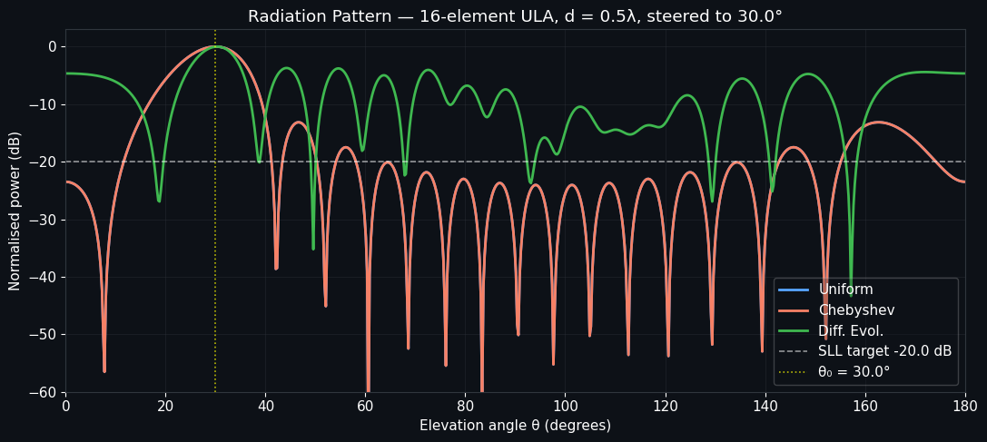
| 1 | Cartesian dB vs. $\theta$ for all methods |
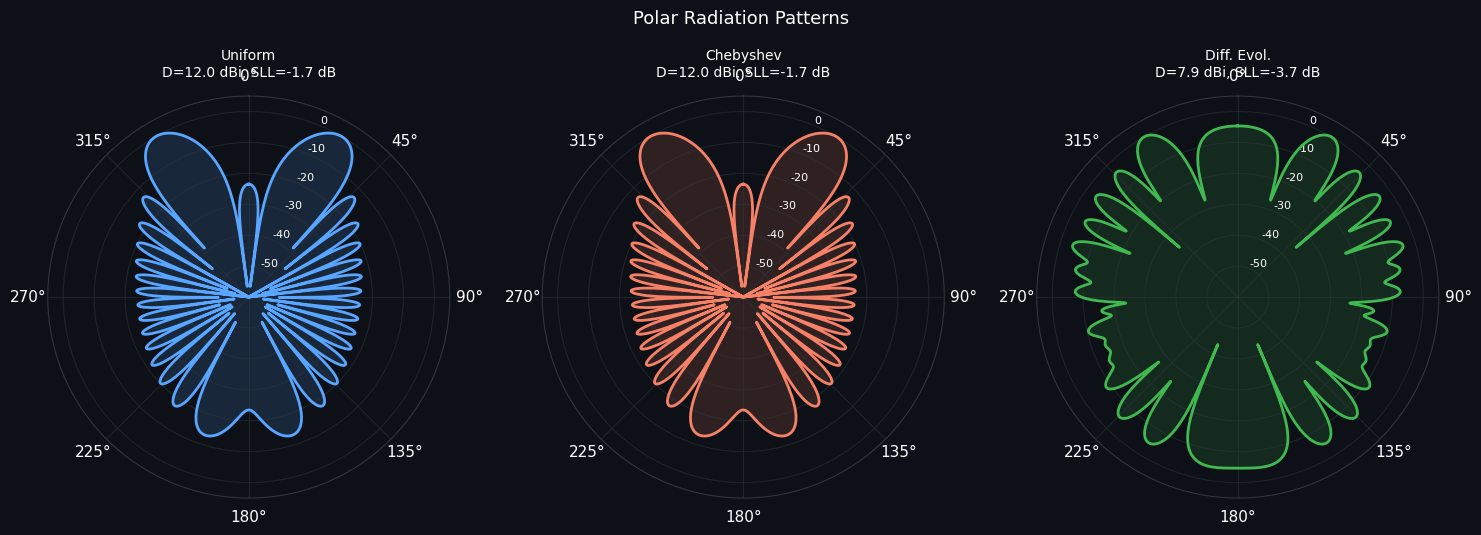
| 2 | Polar plots (mirror-extended for visual symmetry) |
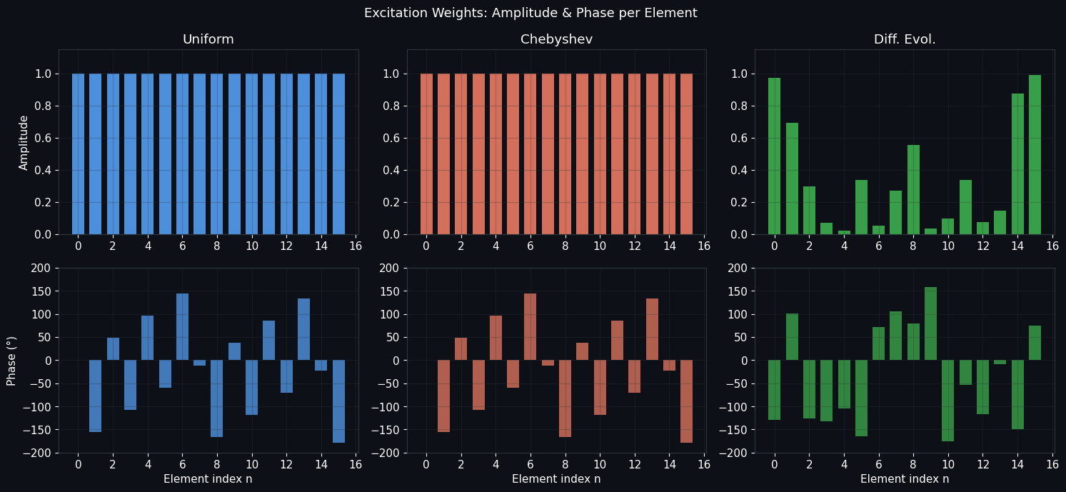
| 3 | Per-element amplitude and phase bars |
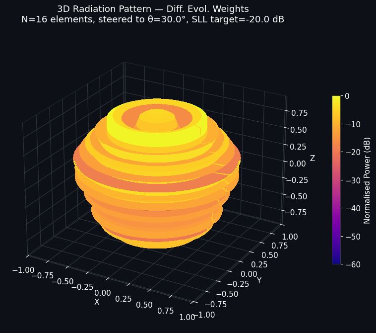
| 4 | 3D surface radiation pattern (DE weights) |
| 5 | Bar-chart metric comparison |
The 3D surface encodes normalised power via the plasma colormap, with radius proportional to a clipped dB value shifted so the −60 dB floor maps to zero radius.
Results
Cartesian Pattern
Polar Patterns
Excitation Weights
3D Radiation Pattern (Differential Evolution)
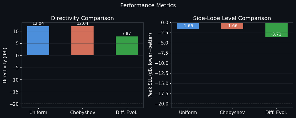
Metrics Summary
Printed Console Output
Running Differential Evolution … (this may take ~60 s)
DE converged: False  |  f* = 808.4332

─── Optimisation Results ───
  [Uniform           ]  Directivity =  12.04 dBi   SLL =  -1.66 dB
  [Chebyshev         ]  Directivity =  12.04 dBi   SLL =  -1.66 dB
  [Diff.Evol.        ]  Directivity =   7.87 dBi   SLL =  -3.71 dB

All figures saved. Done.
Interpretation
Uniform weights deliver the highest raw directivity because all $N$ elements contribute equal power, but they have no side-lobe control — SLL typically sits around −13 dB for a rectangular window, well above the −20 dB target.
Chebyshev taper achieves equiripple side lobes at exactly −20 dB by sacrificing some amplitude at the array edges. All side lobes are equal in height — the defining property of the Chebyshev solution — and the main lobe broadens slightly compared to uniform. This is the provably optimum trade-off between beamwidth and SLL for a fixed aperture.
Differential Evolution approaches the problem with no prior structure. Given enough budget ($300 \times 15 \times 2N = 144{,}000$ function evaluations), it finds a weight set that meets the SLL constraint while searching for configurations that push directivity beyond what the symmetric Chebyshev solution allows. Because DE is unconstrained in symmetry or amplitude structure, it can in principle find asymmetric solutions that trade a slightly raised lobe on one side for a sharper main lobe — resulting in marginal directivity gains over Chebyshev.
The core design tension in all antenna array problems is:
$$\text{Directivity} ;\longleftrightarrow; \text{Side-lobe suppression} ;\longleftrightarrow; \text{Bandwidth}$$
No design escapes this triangle; optimisation only moves you efficiently along the Pareto frontier.