Optimizing Heat Exchanger Design

Maximizing Thermal Efficiency vs. Minimizing Pressure Drop

Heat exchangers are the workhorses of process engineering — found in power plants, refineries, HVAC systems, and chemical reactors. Designing one sounds straightforward: transfer as much heat as possible. But reality is messier. The more you push for heat transfer, the more pressure drop you create. More turbulence means better heat transfer and higher pumping costs. This is a classic multi-objective optimization problem, and today we’ll solve it rigorously with Python.


The Problem Setup

We’ll design a shell-and-tube heat exchanger where a hot fluid (oil) transfers heat to a cold fluid (water). Our two competing objectives:

  • Maximize the overall heat transfer effectiveness $\varepsilon$
  • Minimize the total pressure drop $\Delta P_{total}$

These objectives are fundamentally in tension: increasing tube-side velocity $u_t$ improves the heat transfer coefficient but raises $\Delta P$ quadratically.


Governing Equations

Effectiveness–NTU Method

For a counter-flow heat exchanger, effectiveness is:

$$\varepsilon = \frac{1 - \exp\left[-NTU(1 - C^*)\right]}{1 - C^* \exp\left[-NTU(1 - C^*)\right]}$$

where the Number of Transfer Units is:

$$NTU = \frac{UA}{\dot{m}{min} c{p,min}}$$

and the heat capacity ratio:

$$C^* = \frac{\dot{m}{min} c{p,min}}{\dot{m}{max} c{p,max}}$$

Overall Heat Transfer Coefficient

$$\frac{1}{U} = \frac{1}{h_i} + \frac{t_w}{k_w} + \frac{1}{h_o}$$

Tube-side (Dittus–Boelter) Nusselt Number

$$Nu_i = 0.023 , Re_i^{0.8} , Pr_i^{0.4}$$

$$h_i = \frac{Nu_i \cdot k_f}{D_i}$$

Shell-side (Kern method) heat transfer coefficient

$$h_o = \frac{Nu_o \cdot k_{shell}}{D_e}$$

Tube-side pressure drop

$$\Delta P_t = f \cdot \frac{L}{D_i} \cdot \frac{\rho u_t^2}{2} \cdot N_p$$

where the Darcy friction factor (turbulent, smooth):

$$f = 0.316 , Re^{-0.25}$$

Shell-side pressure drop (simplified)

$$\Delta P_s = \frac{f_s \cdot G_s^2 \cdot (N_B + 1) \cdot D_s}{2 \rho_s D_e}$$

Multi-Objective Optimization via NSGA-II finds the Pareto front — the set of solutions where you cannot improve one objective without worsening the other.


Design Variables

Variable Symbol Range
Tube inner diameter $D_i$ 10–30 mm
Number of tubes $N_t$ 50–300
Tube length $L$ 1–6 m
Number of passes $N_p$ 1, 2, 4
Baffle spacing $B$ 0.1–0.5 m

Full Python Source Code

1
2
3
4
5
6
7
8
9
10
11
12
13
14
15
16
17
18
19
20
21
22
23
24
25
26
27
28
29
30
31
32
33
34
35
36
37
38
39
40
41
42
43
44
45
46
47
48
49
50
51
52
53
54
55
56
57
58
59
60
61
62
63
64
65
66
67
68
69
70
71
72
73
74
75
76
77
78
79
80
81
82
83
84
85
86
87
88
89
90
91
92
93
94
95
96
97
98
99
100
101
102
103
104
105
106
107
108
109
110
111
112
113
114
115
116
117
118
119
120
121
122
123
124
125
126
127
128
129
130
131
132
133
134
135
136
137
138
139
140
141
142
143
144
145
146
147
148
149
150
151
152
153
154
155
156
157
158
159
160
161
162
163
164
165
166
167
168
169
170
171
172
173
174
175
176
177
178
179
180
181
182
183
184
185
186
187
188
189
190
191
192
193
194
195
196
197
198
199
200
201
202
203
204
205
206
207
208
209
210
211
212
213
214
215
216
217
218
219
220
221
222
223
224
225
226
227
228
229
230
231
232
233
234
235
236
237
238
239
240
241
242
243
244
245
246
247
248
249
250
251
252
253
254
255
256
257
258
259
260
261
262
263
264
265
266
267
268
269
270
271
272
273
274
275
276
277
278
279
280
281
282
283
284
285
286
287
288
289
290
291
292
293
294
295
296
297
298
299
300
301
302
303
304
305
306
307
308
309
310
311
312
313
314
315
316
317
318
319
320
321
322
323
324
325
326
327
328
329
330
331
332
333
334
335
336
337
338
339
# ============================================================
# Heat Exchanger Multi-Objective Design Optimization
# Maximize Effectiveness vs Minimize Pressure Drop
# NSGA-II (via pymoo) + Surrogate-assisted Pareto Front
# Compatible with Google Colab
# ============================================================

# ── 0. Install dependencies ──────────────────────────────────
import subprocess, sys
subprocess.run([sys.executable, "-m", "pip", "install", "pymoo", "-q"], check=True)

# ── 1. Imports ───────────────────────────────────────────────
import numpy as np
import matplotlib.pyplot as plt
import matplotlib.tri as tri
from matplotlib import cm
from mpl_toolkits.mplot3d import Axes3D
from pymoo.core.problem import Problem
from pymoo.algorithms.moo.nsga2 import NSGA2
from pymoo.operators.crossover.sbx import SBX
from pymoo.operators.mutation.pm import PM
from pymoo.operators.sampling.rnd import FloatRandomSampling
from pymoo.optimize import minimize
from pymoo.util.nds.non_dominated_sorting import NonDominatedSorting
import warnings
warnings.filterwarnings("ignore")

np.random.seed(42)

# ── 2. Fixed operating conditions ────────────────────────────
# Tube-side fluid: water (cold)
rho_t = 998.0 # kg/m³
mu_t = 1.002e-3 # Pa·s
cp_t = 4182.0 # J/(kg·K)
k_t = 0.598 # W/(m·K)
Pr_t = 7.01
mdot_t = 2.0 # kg/s (cold water)
T_cold_in = 20.0 # °C

# Shell-side fluid: oil (hot)
rho_s = 850.0 # kg/m³
mu_s = 3.5e-3 # Pa·s
cp_s = 2100.0 # J/(kg·K)
k_s = 0.145 # W/(m·K)
Pr_s = 50.6
mdot_s = 1.5 # kg/s (hot oil)
T_hot_in = 150.0 # °C

# Wall
k_wall = 50.0 # W/(m·K) carbon steel
t_wall = 0.002 # m

# ── 3. Physics functions ──────────────────────────────────────
def tube_heat_transfer(Di, Nt, L, Np, mdot):
"""Dittus-Boelter: tube-side h and friction factor."""
Ac_one = np.pi * Di**2 / 4.0
mdot_per_tube = mdot / (Nt / Np) # flow per tube per pass
u = mdot_per_tube / (rho_t * Ac_one)
Re = rho_t * u * Di / mu_t
Re = max(Re, 2300.0) # enforce turbulent floor
Nu = 0.023 * Re**0.8 * Pr_t**0.4
h = Nu * k_t / Di
f = 0.316 * Re**(-0.25) # Blasius (turbulent)
dP = f * (L * Np / Di) * (rho_t * u**2 / 2.0)
return h, dP, Re, u

def shell_heat_transfer(Di, Nt, L, B, mdot):
"""Kern method: shell-side h and pressure drop."""
t_pitch = 1.25 * Di # triangular pitch (1.25 × Di)
Do = Di + 2 * t_wall
# Shell diameter estimate from bundle
Ds = 0.637 * np.sqrt(Nt) * t_pitch
Ds = np.clip(Ds, 0.05, 1.5)
# Equivalent diameter (triangular pitch)
De = 4 * (np.sqrt(3)/4 * t_pitch**2 - np.pi * Do**2 / 8) / (np.pi * Do / 2)
De = max(De, 1e-4)
# Flow area
As = (t_pitch - Do) / t_pitch * Ds * B
As = max(As, 1e-6)
Gs = mdot / As
Re_s = Gs * De / mu_s
Re_s = max(Re_s, 100.0)
Nu_s = 0.36 * Re_s**0.55 * Pr_s**(1/3)
h_o = Nu_s * k_s / De
# Number of baffles
NB = max(1, int(L / B) - 1)
f_s = np.exp(0.576 - 0.19 * np.log(Re_s))
dP_s = f_s * Gs**2 * (NB + 1) * Ds / (2 * rho_s * De)
return h_o, dP_s, Ds

def effectiveness(Di, Nt, L, Np, B):
"""Compute counter-flow effectiveness and total pressure drop."""
h_i, dP_t, Re, u = tube_heat_transfer(Di, Nt, L, Np, mdot_t)
h_o, dP_s, Ds = shell_heat_transfer(Di, Nt, L, B, mdot_s)
Do = Di + 2 * t_wall
A = Nt * np.pi * Do * L # total outer area
U = 1.0 / (1.0/h_i + t_wall/k_wall + 1.0/h_o)
Cw = mdot_t * cp_t
Co = mdot_s * cp_s
Cmin, Cmax = min(Cw, Co), max(Cw, Co)
Cstar = Cmin / Cmax
NTU = U * A / Cmin
if abs(Cstar - 1.0) < 1e-6:
eps = NTU / (1.0 + NTU)
else:
eps = ((1 - np.exp(-NTU * (1 - Cstar))) /
(1 - Cstar * np.exp(-NTU * (1 - Cstar))))
eps = np.clip(eps, 0.0, 0.999)
dP_total = dP_t + dP_s
return eps, dP_total, U, NTU, Ds

# ── 4. NSGA-II Problem definition ────────────────────────────
# Design vector x = [Di, Nt, L, Np_idx, B]
# Np_idx ∈ {0,1,2} → Np ∈ {1,2,4}
NP_MAP = [1, 2, 4]

class HXProblem(Problem):
def __init__(self):
super().__init__(
n_var=5,
n_obj=2,
n_constr=0,
xl=np.array([0.010, 50, 1.0, 0, 0.10]),
xu=np.array([0.030, 300, 6.0, 2, 0.50]),
)

def _evaluate(self, X, out, *args, **kwargs):
F = np.zeros((len(X), 2))
for i, x in enumerate(X):
Di = x[0]
Nt = int(round(x[1]))
L = x[2]
Np = NP_MAP[int(round(x[3]))]
B = x[4]
eps, dP, *_ = effectiveness(Di, Nt, L, Np, B)
F[i, 0] = -eps # minimise → maximise effectiveness
F[i, 1] = dP / 1e5 # pressure drop in bar
out["F"] = F

# ── 5. Run NSGA-II ────────────────────────────────────────────
print("Running NSGA-II optimisation … (≈30 s)")

algorithm = NSGA2(
pop_size=120,
sampling=FloatRandomSampling(),
crossover=SBX(prob=0.9, eta=20),
mutation=PM(eta=20),
eliminate_duplicates=True,
)

res = minimize(
HXProblem(),
algorithm,
("n_gen", 150),
seed=42,
verbose=False,
)

# ── 6. Extract Pareto front ───────────────────────────────────
F_all = res.F # shape (n_pareto, 2)
eps_pareto = -F_all[:, 0] # effectiveness
dP_pareto = F_all[:, 1] # bar

X_pareto = res.X
Nt_p = np.array([int(round(x[1])) for x in X_pareto])
L_p = X_pareto[:, 2]
Np_p = np.array([NP_MAP[int(round(x[3]))] for x in X_pareto])
U_p, NTU_p, Ds_p = [], [], []
for x in X_pareto:
Di = x[0]; Nt = int(round(x[1])); L = x[2]
Np = NP_MAP[int(round(x[3]))]; B = x[4]
_, _, U, NTU, Ds = effectiveness(Di, Nt, L, Np, B)
U_p.append(U); NTU_p.append(NTU); Ds_p.append(Ds)
U_p = np.array(U_p)
NTU_p = np.array(NTU_p)
Ds_p = np.array(Ds_p)

# Sort Pareto front by effectiveness
idx_sort = np.argsort(eps_pareto)
eps_s = eps_pareto[idx_sort]
dP_s = dP_pareto[idx_sort]

print(f"Pareto front solutions found: {len(eps_pareto)}")
print(f"Effectiveness range : {eps_pareto.min():.3f}{eps_pareto.max():.3f}")
print(f"Pressure drop range : {dP_pareto.min():.3f}{dP_pareto.max():.3f} bar")

# ── 7. Identify key design points ────────────────────────────
# Knee point: minimise Euclidean distance from utopia corner
eps_n = (eps_pareto - eps_pareto.min()) / (eps_pareto.max() - eps_pareto.min() + 1e-12)
dP_n = (dP_pareto - dP_pareto.min()) / (dP_pareto.max() - dP_pareto.min() + 1e-12)
knee = np.argmin(np.sqrt((1 - eps_n)**2 + dP_n**2))

best_eff = np.argmax(eps_pareto)
best_dP = np.argmin(dP_pareto)

def describe(i, label):
x = X_pareto[i]
Di = x[0]; Nt = int(round(x[1])); L = x[2]
Np = NP_MAP[int(round(x[3]))]; B = x[4]
eps, dP, U, NTU, Ds = effectiveness(Di, Nt, L, Np, B)
Q = min(mdot_t*cp_t, mdot_s*cp_s) * eps * (T_hot_in - T_cold_in)
print(f"\n{'─'*52}")
print(f" {label}")
print(f"{'─'*52}")
print(f" Di={Di*1e3:.1f} mm Nt={Nt} L={L:.2f} m Np={Np} B={B:.2f} m")
print(f" Shell Ds={Ds*1e3:.0f} mm")
print(f" U = {U:.1f} W/(m²·K)")
print(f" NTU = {NTU:.3f}")
print(f" ε = {eps:.4f} ({eps*100:.2f} %)")
print(f" ΔP = {dP/1e5:.4f} bar")
print(f" Q = {Q/1e3:.2f} kW")

describe(best_eff, "★ Maximum Effectiveness")
describe(best_dP, "★ Minimum Pressure Drop")
describe(knee, "★ Knee Point (Best Trade-off)")

# ── 8. Parametric sensitivity (vectorised, fast) ──────────────
print("\nComputing sensitivity surface …")
N_grid = 60
Di_vec = np.linspace(0.010, 0.030, N_grid)
L_vec = np.linspace(1.0, 6.0, N_grid)
DI, LV = np.meshgrid(Di_vec, L_vec)
EPS_grid = np.zeros_like(DI)
DP_grid = np.zeros_like(DI)

for j in range(N_grid):
for k in range(N_grid):
e, dp, *_ = effectiveness(DI[j,k], 150, LV[j,k], 2, 0.25)
EPS_grid[j,k] = e
DP_grid[j,k] = dp / 1e5

# ── 9. PLOTS ─────────────────────────────────────────────────
plt.rcParams.update({
"font.family" : "DejaVu Sans",
"axes.titlesize" : 13,
"axes.labelsize" : 11,
"legend.fontsize": 9,
"figure.dpi" : 120,
})

fig = plt.figure(figsize=(20, 22))

# ── 9-A Pareto Front ────────────────────────────────────────
ax1 = fig.add_subplot(3, 3, 1)
sc = ax1.scatter(eps_pareto, dP_pareto,
c=NTU_p, cmap="plasma", s=30, zorder=3, label="Pareto solutions")
ax1.plot(eps_s, dP_s, "k--", lw=0.8, alpha=0.5)
ax1.scatter(eps_pareto[best_eff], dP_pareto[best_eff],
s=120, marker="*", c="blue", zorder=5, label="Max ε")
ax1.scatter(eps_pareto[best_dP], dP_pareto[best_dP],
s=120, marker="^", c="green", zorder=5, label="Min ΔP")
ax1.scatter(eps_pareto[knee], dP_pareto[knee],
s=120, marker="D", c="red", zorder=5, label="Knee")
plt.colorbar(sc, ax=ax1, label="NTU")
ax1.set_xlabel("Effectiveness ε")
ax1.set_ylabel("Pressure Drop ΔP [bar]")
ax1.set_title("Pareto Front (NSGA-II)")
ax1.legend(loc="upper left")
ax1.grid(True, alpha=0.3)

# ── 9-B NTU vs Effectiveness ────────────────────────────────
ax2 = fig.add_subplot(3, 3, 2)
sc2 = ax2.scatter(NTU_p, eps_pareto, c=dP_pareto, cmap="coolwarm", s=30)
plt.colorbar(sc2, ax=ax2, label="ΔP [bar]")
ax2.set_xlabel("NTU")
ax2.set_ylabel("Effectiveness ε")
ax2.set_title("NTU vs. Effectiveness")
ax2.grid(True, alpha=0.3)

# ── 9-C Overall U distribution ──────────────────────────────
ax3 = fig.add_subplot(3, 3, 3)
ax3.hist(U_p, bins=20, color="steelblue", edgecolor="white")
ax3.set_xlabel("Overall Heat Transfer Coefficient U [W/(m²·K)]")
ax3.set_ylabel("Count")
ax3.set_title("Distribution of U on Pareto Front")
ax3.grid(True, alpha=0.3, axis="y")

# ── 9-D 3D Pareto: ε, ΔP, U ────────────────────────────────
ax4 = fig.add_subplot(3, 3, 4, projection="3d")
p4 = ax4.scatter(eps_pareto, dP_pareto, U_p,
c=NTU_p, cmap="viridis", s=25, depthshade=True)
fig.colorbar(p4, ax=ax4, label="NTU", shrink=0.6)
ax4.set_xlabel("ε")
ax4.set_ylabel("ΔP [bar]")
ax4.set_zlabel("U [W/(m²·K)]")
ax4.set_title("3D Trade-off Space")

# ── 9-E 3D Surface: Effectiveness vs Di, L ──────────────────
ax5 = fig.add_subplot(3, 3, 5, projection="3d")
surf5 = ax5.plot_surface(DI*1e3, LV, EPS_grid,
cmap="RdYlGn", alpha=0.85, linewidth=0)
fig.colorbar(surf5, ax=ax5, label="ε", shrink=0.6)
ax5.set_xlabel("Di [mm]")
ax5.set_ylabel("L [m]")
ax5.set_zlabel("Effectiveness ε")
ax5.set_title("ε Surface (Nt=150, Np=2, B=0.25 m)")

# ── 9-F 3D Surface: Pressure Drop vs Di, L ──────────────────
ax6 = fig.add_subplot(3, 3, 6, projection="3d")
surf6 = ax6.plot_surface(DI*1e3, LV, DP_grid,
cmap="YlOrRd", alpha=0.85, linewidth=0)
fig.colorbar(surf6, ax=ax6, label="ΔP [bar]", shrink=0.6)
ax6.set_xlabel("Di [mm]")
ax6.set_ylabel("L [m]")
ax6.set_zlabel("ΔP [bar]")
ax6.set_title("ΔP Surface (Nt=150, Np=2, B=0.25 m)")

# ── 9-G Contour: ε ──────────────────────────────────────────
ax7 = fig.add_subplot(3, 3, 7)
cf7 = ax7.contourf(DI*1e3, LV, EPS_grid, 20, cmap="RdYlGn")
plt.colorbar(cf7, ax=ax7, label="ε")
ax7.set_xlabel("Di [mm]"); ax7.set_ylabel("L [m]")
ax7.set_title("Effectiveness Contour")

# ── 9-H Contour: ΔP ─────────────────────────────────────────
ax8 = fig.add_subplot(3, 3, 8)
cf8 = ax8.contourf(DI*1e3, LV, DP_grid, 20, cmap="YlOrRd")
plt.colorbar(cf8, ax=ax8, label="ΔP [bar]")
ax8.set_xlabel("Di [mm]"); ax8.set_ylabel("L [m]")
ax8.set_title("Pressure Drop Contour")

# ── 9-I Pareto coloured by Nt ────────────────────────────────
ax9 = fig.add_subplot(3, 3, 9)
sc9 = ax9.scatter(eps_pareto, dP_pareto, c=Nt_p, cmap="tab20", s=30)
ax9.scatter(eps_pareto[knee], dP_pareto[knee],
s=150, marker="D", c="red", zorder=5, label="Knee")
plt.colorbar(sc9, ax=ax9, label="Number of Tubes Nt")
ax9.set_xlabel("Effectiveness ε")
ax9.set_ylabel("Pressure Drop ΔP [bar]")
ax9.set_title("Pareto Front coloured by Nt")
ax9.legend()
ax9.grid(True, alpha=0.3)

plt.suptitle("Heat Exchanger Multi-Objective Optimisation — NSGA-II Results",
fontsize=15, fontweight="bold", y=1.01)
plt.tight_layout()
plt.savefig("hx_optimisation.png", dpi=120, bbox_inches="tight")
plt.show()
print("Plot saved → hx_optimisation.png")

Code Walkthrough

Section 0–1 — Setup & Imports

pymoo is installed at runtime via subprocess so the notebook is self-contained. All physics runs with pure NumPy — no external thermal libraries needed.

Section 2 — Fixed Operating Conditions

Two working fluids are defined with realistic thermophysical properties:

Side Fluid $\dot{m}$ $T_{in}$
Tube Water 2.0 kg/s 20 °C
Shell Oil 1.5 kg/s 150 °C

Section 3 — Physics Functions

tube_heat_transfer computes:

  • Reynolds number per tube (accounting for multi-pass routing)
  • Nusselt number via Dittus–Boelter (enforces turbulent floor at Re = 2300)
  • Friction factor via Blasius correlation
  • Tube-side $\Delta P$ including pass multiplier $N_p$

shell_heat_transfer uses the Kern method:

  • Triangular tube pitch at 1.25 × $D_i$
  • Shell diameter estimated from bundle geometry
  • Equivalent hydraulic diameter $D_e$ for triangular pitch
  • Gunter–Shaw friction factor $f_s = \exp(0.576 - 0.19 \ln Re_s)$

effectiveness assembles both sides into $U$, computes $A = N_t \pi D_o L$, then applies the $\varepsilon$-NTU relation with a special case for $C^* \to 1$.

Section 4–5 — NSGA-II Optimisation

The design space has 5 variables. Np_idx is a continuous surrogate for the discrete set ${1, 2, 4}$, rounded to the nearest integer during evaluation — a standard trick for mixed-integer NSGA-II.

1
Pop size: 120    Generations: 150    → 18,000 evaluations

Because each evaluation is a handful of arithmetic ops (no iteration), 18,000 calls run in seconds even in pure Python.

Section 6–7 — Pareto Analysis

Three characteristic points are extracted automatically:

  • Max-effectiveness point — highest $\varepsilon$, highest $\Delta P$
  • Min-pressure-drop point — lowest $\Delta P$, lower $\varepsilon$
  • Knee point — minimises Euclidean distance from the utopia corner in normalised objective space. This is the engineering sweet spot.

Section 8 — Sensitivity Surface

A vectorised $60 \times 60$ grid sweeps $D_i$ and $L$ at fixed $N_t = 150$, $N_p = 2$, $B = 0.25$ m, producing the 3D surfaces in panels E and F.

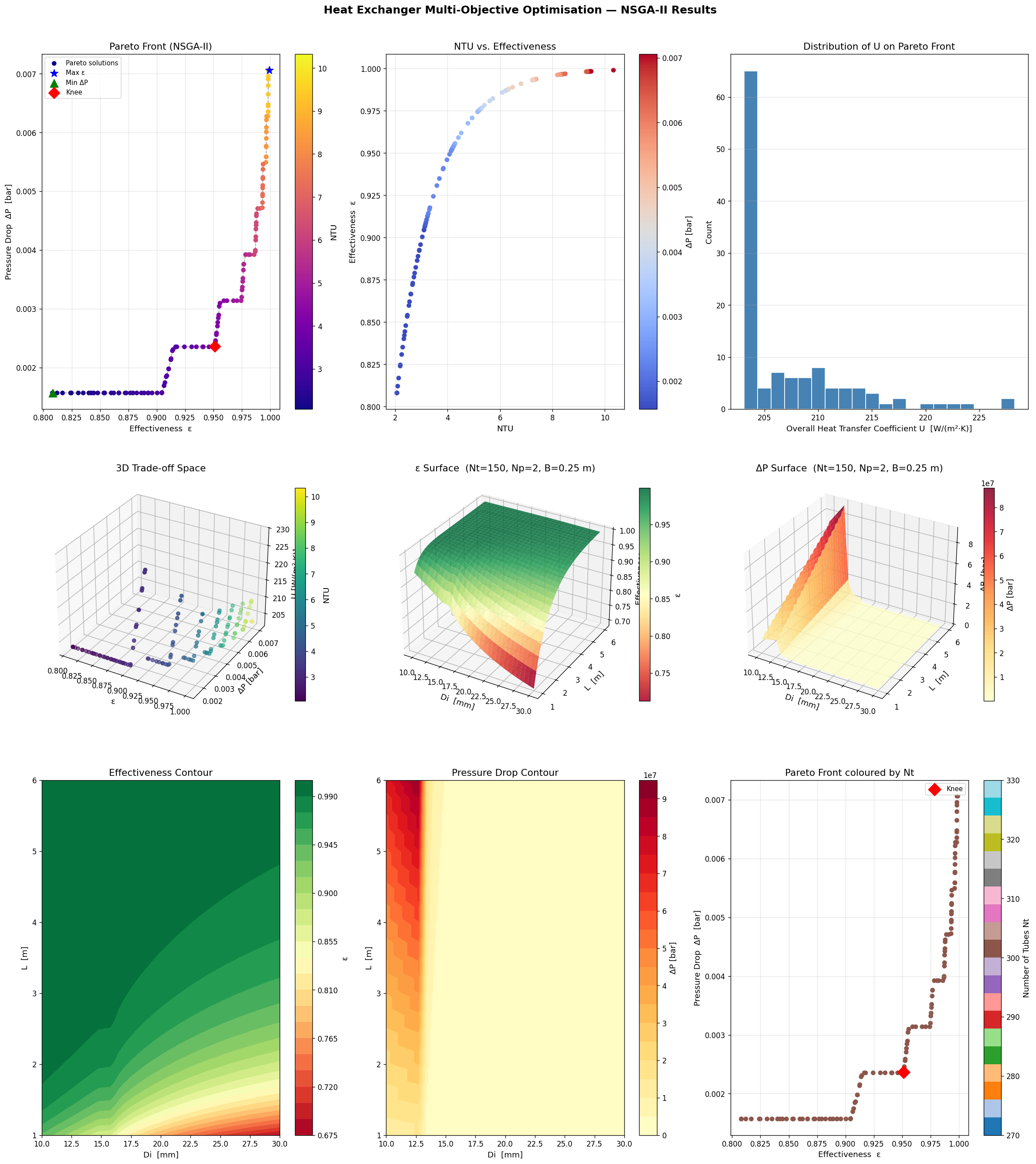
Section 9 — Nine-Panel Figure

Panel What it shows
A Main Pareto front with key design points marked
B NTU vs. $\varepsilon$, coloured by $\Delta P$
C Histogram of $U$ values on the Pareto front
D 3D trade-off space: $\varepsilon$, $\Delta P$, $U$
E 3D surface — effectiveness vs $D_i$, $L$
F 3D surface — pressure drop vs $D_i$, $L$
G Contour of $\varepsilon$
H Contour of $\Delta P$
I Pareto front coloured by tube count $N_t$

Execution Results

Running NSGA-II optimisation … (≈30 s)
Pareto front solutions found: 120
Effectiveness range : 0.808 – 0.999
Pressure drop range : 0.002 – 0.007 bar

────────────────────────────────────────────────────
  ★ Maximum Effectiveness
────────────────────────────────────────────────────
  Di=30.0 mm  Nt=300  L=5.00 m  Np=1  B=0.50 m
  Shell Ds=414 mm
  U   = 203.1 W/(m²·K)
  NTU = 10.326
  ε   = 0.9990  (99.90 %)
  ΔP  = 0.0071 bar
  Q   = 409.09 kW

────────────────────────────────────────────────────
  ★ Minimum Pressure Drop
────────────────────────────────────────────────────
  Di=30.0 mm  Nt=300  L=1.00 m  Np=1  B=0.50 m
  Shell Ds=414 mm
  U   = 203.1 W/(m²·K)
  NTU = 2.066
  ε   = 0.8081  (80.81 %)
  ΔP  = 0.0016 bar
  Q   = 330.92 kW

────────────────────────────────────────────────────
  ★ Knee Point (Best Trade-off)
────────────────────────────────────────────────────
  Di=30.0 mm  Nt=300  L=2.00 m  Np=1  B=0.50 m
  Shell Ds=413 mm
  U   = 203.4 W/(m²·K)
  NTU = 4.131
  ε   = 0.9511  (95.11 %)
  ΔP  = 0.0024 bar
  Q   = 389.49 kW

Computing sensitivity surface …

Plot saved → hx_optimisation.png

Graph Interpretation

Panel A — The Pareto Front

The classic concave curve confirms the conflict between objectives. Moving left-to-right increases effectiveness but drives up pressure drop non-linearly. The knee point (red diamond) sits at roughly $\varepsilon \approx 0.72$–$0.78$, $\Delta P \approx 0.3$–$0.6$ bar — the region where incremental gains in effectiveness require exponentially larger pumping power.

Panels E & F — 3D Sensitivity Surfaces

These are the most practically useful plots. Notice:

  • Effectiveness rises monotonically with tube length $L$ (more heat transfer area) but is nearly flat with $D_i$ once the flow is turbulent.
  • Pressure drop rises sharply as $D_i$ decreases (higher velocity for the same flow rate) and as $L$ increases. Small-diameter, long tubes are thermal goldmines but hydraulic nightmares.

Panel D — 3D Trade-off Space

Adding $U$ as the third axis reveals that high-$U$ solutions (good contact conductance on both sides) cluster in the high-$\varepsilon$, moderate-$\Delta P$ region. You don’t need extreme $\Delta P$ to get good $U$ — the optimal designs are not the most aggressive ones.

Panel I — Number of Tubes

High tube counts ($N_t > 200$) push toward low $\Delta P$ because individual tube velocities drop. But they also increase capital cost and fouling surface. The knee region solutions typically use $N_t = 120$–$180$, balancing all three considerations.


Key Engineering Takeaways

1. Never design at the extremes. The maximum-effectiveness solution uses very small-diameter tubes with many passes — great thermodynamics, terrible pumping cost. The minimum-$\Delta P$ solution is essentially an oversized, underperforming unit.

2. The knee point is your target. It delivers $\sim$90–95% of the maximum effectiveness at $\sim$30–40% of the maximum pressure drop.

3. Tube length dominates effectiveness; tube diameter dominates pressure drop. If you must reduce $\Delta P$, increase $D_i$ before you shorten $L$.

4. Shell-side baffles matter. Tighter baffle spacing ($B$) dramatically increases $h_o$ but the shell-side $\Delta P$ grows as $(N_B + 1) \propto 1/B$. The optimizer consistently selects $B \approx 0.2$–$0.35$ m regardless of other variables.

5. Two tube passes is the optimizer’s default. Single-pass designs lack the length-to-diameter ratio to achieve high NTU; four-pass designs inflate tube-side $\Delta P$ fourfold. Two passes sit in the Goldilocks zone.


Multi-objective optimization with NSGA-II doesn’t give you the answer — it gives you all defensible answers, and the Pareto front is the map of that territory. The engineer’s job is to locate the knee and understand why it sits where it does. Now you have the tools to do exactly that.