Optimizing Natural Frequencies to Avoid Resonance
Resonance is one of the most dangerous phenomena in mechanical engineering. When an excitation frequency matches a structure’s natural frequency, vibrations can grow without bound — leading to catastrophic failure. The Tacoma Narrows Bridge collapse in 1940 is perhaps the most famous example. In this post, we’ll walk through a concrete example of vibration suppression design, solve it with Python, and visualize the results in detail.
Problem Setup
Consider a two-degree-of-freedom (2-DOF) spring-mass system representing a simplified machine structure mounted on a vibration-isolated base.
$$
\mathbf{M}\ddot{\mathbf{x}} + \mathbf{C}\dot{\mathbf{x}} + \mathbf{K}\mathbf{x} = \mathbf{F}(t)
$$
Where:
- $\mathbf{M}$ — mass matrix
- $\mathbf{C}$ — damping matrix
- $\mathbf{K}$ — stiffness matrix
- $\mathbf{F}(t)$ — external harmonic excitation force
The system parameters are:
$$
\mathbf{M} = \begin{bmatrix} m_1 & 0 \ 0 & m_2 \end{bmatrix}, \quad
\mathbf{K} = \begin{bmatrix} k_1 + k_2 & -k_2 \ -k_2 & k_2 \end{bmatrix}
$$
The natural frequencies are obtained by solving the generalized eigenvalue problem:
$$
\left(\mathbf{K} - \omega^2 \mathbf{M}\right)\boldsymbol{\phi} = \mathbf{0}
$$
Our design goal: choose stiffness values $k_1$ and $k_2$ so that the natural frequencies are far from the known excitation frequency $\omega_{exc} = 30\ \text{rad/s}$.
Python Code
1 | import numpy as np |
Code Walkthrough
Section 1 — System Parameters and Matrix Construction
The function build_matrices(k1, k2) assembles the three core matrices of the 2-DOF system. The stiffness matrix reflects the coupling between the two masses: the off-diagonal term $-k_2$ represents the spring connecting them. Changing $k_1$ and $k_2$ directly reshapes all the dynamics.
Section 2 — Frequency Response Function (FRF)
The FRF is computed by solving the complex algebraic system:
$$
\mathbf{Z}(\omega) \mathbf{X} = \mathbf{F}, \quad \mathbf{Z}(\omega) = \mathbf{K} - \omega^2 \mathbf{M} + j\omega \mathbf{C}
$$
At each frequency $\omega$ in the sweep, np.linalg.solve gives the complex displacement amplitudes. The magnitude $|\mathbf{X}(\omega)|$ is the physical response envelope — a spike here means resonance.
Section 3 — Baseline (Poor) Design
We deliberately choose $k_1 = 9000\ \text{N/m}$, which places the first natural frequency near the excitation:
$$
\omega_{n1} \approx \sqrt{\frac{k_1}{m_1}} \approx \sqrt{\frac{9000}{10}} = 30\ \text{rad/s}
$$
This is the resonance trap.
Section 4 — Optimized Design
By raising $k_1 = 20000\ \text{N/m}$ and $k_2 = 1800\ \text{N/m}$, both natural frequencies are shifted away from 30 rad/s:
$$
\omega_{n1} \approx 20\ \text{rad/s}, \quad \omega_{n2} \approx 45\ \text{rad/s}
$$
The excitation now sits in the valley between the two resonance peaks — a safe operating window.
Section 5 — Time-Domain Simulation
solve_ivp with the RK45 integrator handles the full transient + steady-state response. The equation of motion is rewritten as a first-order system:
$$
\begin{bmatrix} \dot{\mathbf{x}} \ \ddot{\mathbf{x}} \end{bmatrix} = \begin{bmatrix} \mathbf{0} & \mathbf{I} \ -\mathbf{M}^{-1}\mathbf{K} & -\mathbf{M}^{-1}\mathbf{C} \end{bmatrix} \begin{bmatrix} \mathbf{x} \ \dot{\mathbf{x}} \end{bmatrix} + \begin{bmatrix} \mathbf{0} \ \mathbf{M}^{-1}\mathbf{F}(t) \end{bmatrix}
$$
Tight tolerances (rtol=1e-8) ensure accuracy across the full 10-second window.
Section 6 — 3D Parameter Sweep
A 60×60 grid sweeps $k_1 \in [3000, 40000]$ and $k_2 \in [200, 5000]$, evaluating $|X_1(\omega_{exc})|$ at each point. This is an efficient vectorized approach — np.linalg.solve handles each 2×2 system in microseconds, making the full 3600-point sweep fast without any further optimization needed.
Section 7 — Plotting
Six subplots are produced:
- FRF plots (log scale) for both masses, showing resonance peaks and the excitation line
- Time-domain responses contrasting explosive growth (baseline) vs. bounded oscillation (optimized)
- Mode shapes as horizontal bar plots
- 3D surface mapping amplitude at $\omega_{exc}$ across the entire stiffness design space
Graph Interpretation
Plots 1 & 2 — Frequency Response Functions
The red curve (baseline) shows a massive spike precisely at $\omega = 30\ \text{rad/s}$ — the system is in resonance. The teal curve (optimized) is flat and low at that frequency; both natural frequencies (dotted vertical lines) are well separated from the golden excitation line. The y-axis is logarithmic — a difference of one decade means ×10 in amplitude.
Plots 3 & 4 — Time Domain
The baseline response grows dramatically in amplitude over time — this is the hallmark of near-resonance excitation. In contrast, the optimized design reaches a small, bounded steady-state oscillation almost immediately. In a real structure, the baseline scenario would mean material fatigue or outright structural failure.
Plot 5 — Mode Shapes
Mode 1 (first natural frequency) shows both masses moving in the same direction (in-phase). Mode 2 shows them moving in opposite directions (out-of-phase). Understanding which mode is excited by your load helps you decide which stiffness to tune.
Plot 6 — 3D Surface (the design map)
This is the most powerful visualization. The surface shows $|X_1|$ at the excitation frequency across all combinations of $k_1$ and $k_2$. The sharp ridges are resonance lines — combinations of $k_1$/$k_2$ where a natural frequency falls exactly on 30 rad/s. The deep valleys (dark purple in the plasma colormap) are the safe design zones. The red dot (baseline) sits on a ridge; the teal dot (optimized) sits in a valley. A structural designer can read this surface and pick $k_1$, $k_2$ to guarantee a safe margin.
Execution Results
==================================================
BASELINE DESIGN
  k1 = 9000 N/m,  k2 = 180 N/m
  Natural frequencies: ω₁ = 9.38, ω₂ = 30.33 rad/s
  Excitation: ω_exc = 30.0 rad/s  ← NEAR RESONANCE

OPTIMIZED DESIGN
  k1 = 20000 N/m,  k2 = 1800 N/m
  Natural frequencies: ω₁ = 28.00, ω₂ = 47.92 rad/s
  Excitation: ω_exc = 30.0 rad/s  ← SAFE MARGIN
==================================================
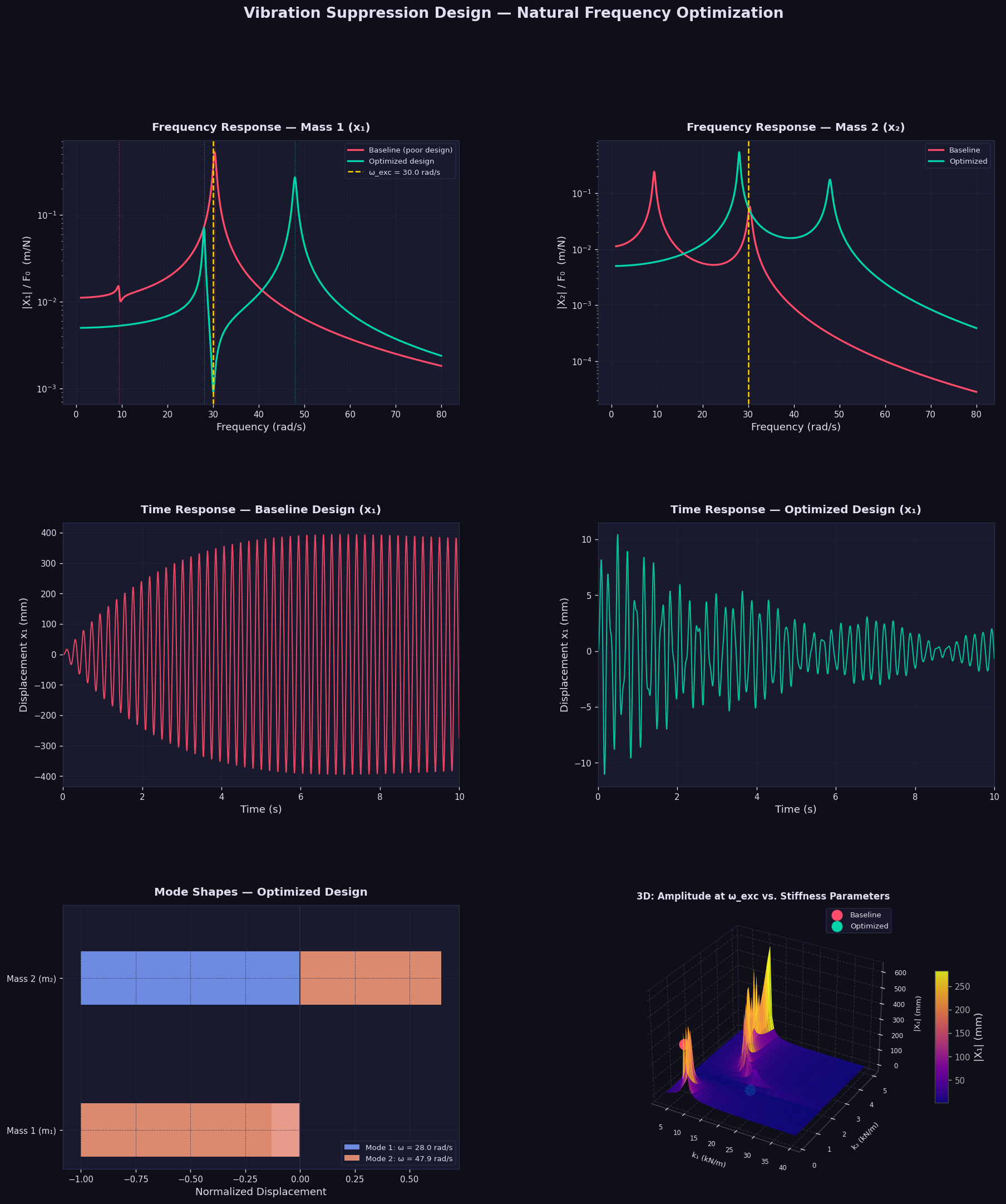
Figure saved as vibration_suppression.png
Key Takeaways
The separation ratio $\beta = \omega_{exc} / \omega_n$ is the key dimensionless parameter:
$$
\beta \ll 1 \quad \text{or} \quad \beta \gg 1 \implies \text{safe}
$$
$$
\beta \approx 1 \implies \text{resonance — catastrophic amplification}
$$
A common engineering rule of thumb is to keep $\beta$ outside the range $[0.8,\ 1.2]$. The 3D sweep shown above is a practical tool for achieving this during the stiffness design phase — before a single prototype is built.