Cross-Section Shape Optimization of a Beam

Minimizing Deflection While Reducing Material Usage

Structural optimization is one of the most compelling intersections of engineering mechanics, mathematics, and modern computation. In this article, we tackle a classic structural engineering problem: how to optimally shape the cross-section of a simply supported beam so that it deflects as little as possible under a given load, while simultaneously using as little material as possible. We’ll solve this with Python using scipy.optimize, visualize the geometry in 2D and 3D, and walk through every step of the math and code.


Problem Setup

Consider a simply supported beam of length $L$ subjected to a uniformly distributed load $q$ (N/m). We want to choose the width $b$ and height $h$ of a solid rectangular cross-section to:

Minimize the maximum midspan deflection:

$$\delta_{\max} = \frac{5 q L^4}{384 E I}$$

where the second moment of area for a rectangle is:

$$I = \frac{b h^3}{12}$$

Subject to constraints:

  1. Volume (material) constraint — cross-sectional area $A = b \cdot h$ must not exceed a prescribed limit $A_{\max}$:

$$b \cdot h \leq A_{\max}$$

  1. Bending stress constraint — the maximum bending stress must not exceed the allowable stress $\sigma_{\text{allow}}$:

$$\sigma_{\max} = \frac{M_{\max} \cdot (h/2)}{I} \leq \sigma_{\text{allow}}, \quad M_{\max} = \frac{q L^2}{8}$$

  1. Geometric bounds — practical lower and upper limits on $b$ and $h$:

$$b_{\min} \leq b \leq b_{\max}, \quad h_{\min} \leq h \leq h_{\max}$$

The design variables are $\mathbf{x} = [b, h]$.


Why Is $h$ More Valuable Than $b$?

Notice that $I \propto h^3$ but only $\propto b^1$. This means increasing the height is cubically more effective at reducing deflection than increasing the width by the same amount. The optimizer should discover this naturally — and push $h$ to its upper limit while keeping $b$ lean.

This is exactly why I-beams and T-beams are shaped the way they are in real structures.


The Optimization Problem in Standard Form

$$\min_{b,h} ; f(b,h) = \frac{5 q L^4}{384 E} \cdot \frac{12}{b h^3} = \frac{5 q L^4 \cdot 12}{384 E \cdot b h^3}$$

$$\text{subject to:} \quad g_1: ; bh - A_{\max} \leq 0$$

$$g_2: ; \frac{q L^2}{8} \cdot \frac{6}{b h^2} - \sigma_{\text{allow}} \leq 0$$

$$b_{\min} \leq b \leq b_{\max}, \quad h_{\min} \leq h \leq h_{\max}$$

We will use scipy.optimize.minimize with the SLSQP (Sequential Least Squares Programming) method, which handles nonlinear constraints and bound constraints natively.


Full Source Code

1
2
3
4
5
6
7
8
9
10
11
12
13
14
15
16
17
18
19
20
21
22
23
24
25
26
27
28
29
30
31
32
33
34
35
36
37
38
39
40
41
42
43
44
45
46
47
48
49
50
51
52
53
54
55
56
57
58
59
60
61
62
63
64
65
66
67
68
69
70
71
72
73
74
75
76
77
78
79
80
81
82
83
84
85
86
87
88
89
90
91
92
93
94
95
96
97
98
99
100
101
102
103
104
105
106
107
108
109
110
111
112
113
114
115
116
117
118
119
120
121
122
123
124
125
126
127
128
129
130
131
132
133
134
135
136
137
138
139
140
141
142
143
144
145
146
147
148
149
150
151
152
153
154
155
156
157
158
159
160
161
162
163
164
165
166
167
168
169
170
171
172
173
174
175
176
177
178
179
180
181
182
183
184
185
186
187
188
189
190
191
192
193
194
195
196
197
198
199
200
201
202
203
204
205
206
207
208
209
210
211
212
213
214
215
216
217
218
219
220
221
222
223
224
225
226
227
228
229
230
231
232
233
234
235
236
237
238
239
240
241
242
243
244
245
246
247
248
249
250
251
252
253
254
255
256
257
258
259
260
261
262
263
264
265
266
267
268
269
270
271
272
273
274
275
276
277
278
279
280
281
282
283
284
285
286
287
288
289
290
291
292
293
294
295
296
297
298
299
300
301
302
303
304
305
306
307
308
309
310
311
312
313
314
315
316
317
318
319
320
321
322
323
324
325
326
327
328
329
330
331
332
333
334
335
336
337
338
339
340
341
342
343
344
345
346
347
348
349
350
351
352
353
354
355
356
357
358
359
360
361
362
363
364
365
366
367
368
369
370
371
372
# ============================================================
# Beam Cross-Section Shape Optimization
# Minimize midspan deflection subject to material and stress
# constraints on a simply supported rectangular beam.
# Environment: Google Colaboratory
# ============================================================

import numpy as np
import matplotlib.pyplot as plt
import matplotlib.patches as patches
from matplotlib import cm
from mpl_toolkits.mplot3d import Axes3D
from scipy.optimize import minimize, differential_evolution
import warnings
warnings.filterwarnings("ignore")

# ─────────────────────────────────────────
# 1. Problem Parameters
# ─────────────────────────────────────────
L = 5.0 # Beam length [m]
q = 10_000.0 # Uniformly distributed load [N/m]
E = 200e9 # Young's modulus (steel) [Pa]
sigma_al = 150e6 # Allowable bending stress [Pa]
A_max = 0.012 # Max cross-sectional area [m^2]

# Design variable bounds: [b_min, b_max], [h_min, h_max]
b_min, b_max = 0.05, 0.40
h_min, h_max = 0.10, 0.80

# ─────────────────────────────────────────
# 2. Engineering Functions
# ─────────────────────────────────────────
def second_moment(b, h):
"""Second moment of area for a rectangle."""
return b * h**3 / 12.0

def deflection(b, h):
"""Maximum midspan deflection under UDL."""
I = second_moment(b, h)
return (5 * q * L**4) / (384 * E * I)

def bending_stress(b, h):
"""Maximum bending stress at midspan."""
I = second_moment(b, h)
M = q * L**2 / 8.0
return M * (h / 2.0) / I

def area(b, h):
return b * h

# ─────────────────────────────────────────
# 3. Objective and Constraints for SLSQP
# ─────────────────────────────────────────
def objective(x):
b, h = x
return deflection(b, h)

constraints = [
# g1: area ≤ A_max → A_max - area ≥ 0
{"type": "ineq", "fun": lambda x: A_max - area(x[0], x[1])},
# g2: stress ≤ sigma_al → sigma_al - stress ≥ 0
{"type": "ineq", "fun": lambda x: sigma_al - bending_stress(x[0], x[1])},
]

bounds = [(b_min, b_max), (h_min, h_max)]

# ─────────────────────────────────────────
# 4. Multi-Start SLSQP (avoid local minima)
# ─────────────────────────────────────────
np.random.seed(42)
best_result = None
best_val = np.inf

n_starts = 60
for _ in range(n_starts):
b0 = np.random.uniform(b_min, b_max)
h0 = np.random.uniform(h_min, h_max)
x0 = [b0, h0]
try:
res = minimize(objective, x0,
method="SLSQP",
bounds=bounds,
constraints=constraints,
options={"ftol": 1e-12, "maxiter": 2000})
if res.success and res.fun < best_val:
best_val = res.fun
best_result = res
except Exception:
pass

b_opt, h_opt = best_result.x
d_opt = deflection(b_opt, h_opt)
s_opt = bending_stress(b_opt, h_opt)
A_opt = area(b_opt, h_opt)
I_opt = second_moment(b_opt, h_opt)

print("=" * 52)
print(" OPTIMIZATION RESULTS")
print("=" * 52)
print(f" Optimal width b* = {b_opt*100:.4f} cm")
print(f" Optimal height h* = {h_opt*100:.4f} cm")
print(f" Section area A* = {A_opt*1e4:.4f} cm²")
print(f" Second moment I* = {I_opt*1e8:.6f} cm⁴ (×10⁻⁸ m⁴)")
print(f" Max deflection δ* = {d_opt*1000:.6f} mm")
print(f" Max stress σ* = {s_opt/1e6:.4f} MPa")
print(f" Area constraint : {A_opt:.6f}{A_max:.6f}")
print(f" Stress constraint: {s_opt/1e6:.4f}{sigma_al/1e6:.1f} MPa")
print("=" * 52)

# ─────────────────────────────────────────
# 5. Baseline: square section of same area
# ─────────────────────────────────────────
b_sq = h_sq = np.sqrt(A_max)
d_sq = deflection(b_sq, h_sq)
s_sq = bending_stress(b_sq, h_sq)
print(f"\n [Baseline – square section, A = A_max]")
print(f" b = h = {b_sq*100:.4f} cm")
print(f" δ = {d_sq*1000:.6f} mm")
print(f" σ = {s_sq/1e6:.4f} MPa")
print(f" Deflection improvement: {(1 - d_opt/d_sq)*100:.1f}%")

# ─────────────────────────────────────────
# 6. Visualizations
# ─────────────────────────────────────────
plt.style.use("dark_background")
CMAP = cm.plasma
fig = plt.figure(figsize=(20, 18))
fig.patch.set_facecolor("#0d0d0d")

# ── 6-A Cross-section comparison ─────────────────────────
ax1 = fig.add_subplot(3, 3, 1)
ax1.set_facecolor("#111111")
ax1.set_aspect("equal")

# Square baseline
rect_sq = patches.Rectangle(
(-b_sq/2, -h_sq/2), b_sq, h_sq,
linewidth=2, edgecolor="#888888", facecolor="#333333", label="Square baseline")
ax1.add_patch(rect_sq)

# Optimal section
rect_op = patches.Rectangle(
(-b_opt/2, -h_opt/2), b_opt, h_opt,
linewidth=2, edgecolor="#ff6f3c", facecolor="none",
linestyle="--", label="Optimal section")
ax1.add_patch(rect_op)

margin = 0.05
ax1.set_xlim(-b_max/2 - margin, b_max/2 + margin)
ax1.set_ylim(-h_max/2 - margin, h_max/2 + margin)
ax1.set_title("Cross-Section Comparison", color="white", fontsize=11)
ax1.set_xlabel("Width b [m]", color="#aaaaaa")
ax1.set_ylabel("Height h [m]", color="#aaaaaa")
ax1.tick_params(colors="#aaaaaa")
ax1.legend(fontsize=8, facecolor="#222222", edgecolor="#555555", labelcolor="white")
for sp in ax1.spines.values():
sp.set_edgecolor("#333333")

# ── 6-B Deflection surface ────────────────────────────────
ax2 = fig.add_subplot(3, 3, 2, projection="3d")
ax2.set_facecolor("#0d0d0d")

B_g = np.linspace(b_min, b_max, 60)
H_g = np.linspace(h_min, h_max, 60)
B_m, H_m = np.meshgrid(B_g, H_g)
D_m = deflection(B_m, H_m) * 1000 # mm

surf = ax2.plot_surface(B_m * 100, H_m * 100, D_m,
cmap=CMAP, alpha=0.85, linewidth=0)
ax2.scatter([b_opt*100], [h_opt*100], [d_opt*1000],
color="#00ffcc", s=120, zorder=10, label="Optimum")
ax2.set_title("Deflection Surface δ (mm)", color="white", fontsize=11, pad=10)
ax2.set_xlabel("b [cm]", color="#aaaaaa", labelpad=6)
ax2.set_ylabel("h [cm]", color="#aaaaaa", labelpad=6)
ax2.set_zlabel("δ [mm]", color="#aaaaaa", labelpad=6)
ax2.tick_params(colors="#aaaaaa")
ax2.xaxis.pane.fill = False
ax2.yaxis.pane.fill = False
ax2.zaxis.pane.fill = False
cbar2 = fig.colorbar(surf, ax=ax2, shrink=0.5, pad=0.1)
cbar2.ax.yaxis.set_tick_params(color="#aaaaaa")
plt.setp(cbar2.ax.yaxis.get_ticklabels(), color="#aaaaaa")

# ── 6-C Stress surface ───────────────────────────────────
ax3 = fig.add_subplot(3, 3, 3, projection="3d")
ax3.set_facecolor("#0d0d0d")

S_m = bending_stress(B_m, H_m) / 1e6 # MPa

surf3 = ax3.plot_surface(B_m * 100, H_m * 100, S_m,
cmap=cm.inferno, alpha=0.85, linewidth=0)
ax3.scatter([b_opt*100], [h_opt*100], [s_opt/1e6],
color="#00ffcc", s=120, zorder=10)
ax3.set_title("Bending Stress Surface σ (MPa)", color="white", fontsize=11, pad=10)
ax3.set_xlabel("b [cm]", color="#aaaaaa", labelpad=6)
ax3.set_ylabel("h [cm]", color="#aaaaaa", labelpad=6)
ax3.set_zlabel("σ [MPa]", color="#aaaaaa", labelpad=6)
ax3.tick_params(colors="#aaaaaa")
ax3.xaxis.pane.fill = False
ax3.yaxis.pane.fill = False
ax3.zaxis.pane.fill = False
cbar3 = fig.colorbar(surf3, ax=ax3, shrink=0.5, pad=0.1)
cbar3.ax.yaxis.set_tick_params(color="#aaaaaa")
plt.setp(cbar3.ax.yaxis.get_ticklabels(), color="#aaaaaa")

# ── 6-D Deflection contour + feasible region ─────────────
ax4 = fig.add_subplot(3, 3, 4)
ax4.set_facecolor("#111111")

D_log = np.log10(D_m)
c4 = ax4.contourf(B_g * 100, H_g * 100, D_log, levels=30, cmap=CMAP)
cbar4 = fig.colorbar(c4, ax=ax4)
cbar4.set_label("log10(δ [mm])", color="#aaaaaa")
cbar4.ax.yaxis.set_tick_params(color="#aaaaaa")
plt.setp(cbar4.ax.yaxis.get_ticklabels(), color="#aaaaaa")

# Overlay constraint boundaries
A_feas = (B_m * H_m <= A_max)
Sig_feas = (bending_stress(B_m, H_m) <= sigma_al)
feasible = A_feas & Sig_feas
ax4.contour(B_g * 100, H_g * 100, (B_m * H_m),
levels=[A_max], colors="#ff6f3c", linewidths=2,
linestyles="--")
ax4.contour(B_g * 100, H_g * 100, bending_stress(B_m, H_m) / 1e6,
levels=[sigma_al / 1e6], colors="#00ffcc", linewidths=2,
linestyles=":")
ax4.plot(b_opt * 100, h_opt * 100, "w*", markersize=14, label="Optimum")
ax4.set_title("Deflection Contour + Constraints", color="white", fontsize=11)
ax4.set_xlabel("b [cm]", color="#aaaaaa")
ax4.set_ylabel("h [cm]", color="#aaaaaa")
ax4.tick_params(colors="#aaaaaa")
ax4.legend(fontsize=8, facecolor="#222222", edgecolor="#555555", labelcolor="white")
for sp in ax4.spines.values():
sp.set_edgecolor("#333333")

# ── 6-E Second moment of area surface ────────────────────
ax5 = fig.add_subplot(3, 3, 5, projection="3d")
ax5.set_facecolor("#0d0d0d")

I_m = second_moment(B_m, H_m) * 1e8 # cm^4

surf5 = ax5.plot_surface(B_m * 100, H_m * 100, I_m,
cmap=cm.viridis, alpha=0.85, linewidth=0)
ax5.scatter([b_opt*100], [h_opt*100], [I_opt*1e8],
color="#ff6f3c", s=120, zorder=10)
ax5.set_title("Second Moment of Area I (×10⁻⁸ m⁴)", color="white", fontsize=11, pad=10)
ax5.set_xlabel("b [cm]", color="#aaaaaa", labelpad=6)
ax5.set_ylabel("h [cm]", color="#aaaaaa", labelpad=6)
ax5.set_zlabel("I [×10⁻⁸ m⁴]", color="#aaaaaa", labelpad=6)
ax5.tick_params(colors="#aaaaaa")
ax5.xaxis.pane.fill = False
ax5.yaxis.pane.fill = False
ax5.zaxis.pane.fill = False
cbar5 = fig.colorbar(surf5, ax=ax5, shrink=0.5, pad=0.1)
cbar5.ax.yaxis.set_tick_params(color="#aaaaaa")
plt.setp(cbar5.ax.yaxis.get_ticklabels(), color="#aaaaaa")

# ── 6-F Trade-off: h vs deflection for fixed area ────────
ax6 = fig.add_subplot(3, 3, 6)
ax6.set_facecolor("#111111")

h_sweep = np.linspace(h_min, h_max, 300)
# For each h, use b = A_max / h (saturate area constraint)
b_sweep = np.clip(A_max / h_sweep, b_min, b_max)
d_sweep = deflection(b_sweep, h_sweep) * 1000

ax6.plot(h_sweep * 100, d_sweep, color="#ff6f3c", linewidth=2,
label="δ along $A = A_{max}$ boundary")
ax6.axvline(h_opt * 100, color="#00ffcc", linestyle="--", linewidth=1.5,
label=f"h* = {h_opt*100:.2f} cm")
ax6.axhline(d_opt * 1000, color="white", linestyle=":", linewidth=1,
label=f"δ* = {d_opt*1000:.4f} mm")
ax6.set_title("Trade-off: h vs Deflection (at max area)", color="white", fontsize=11)
ax6.set_xlabel("Height h [cm]", color="#aaaaaa")
ax6.set_ylabel("Deflection δ [mm]", color="#aaaaaa")
ax6.tick_params(colors="#aaaaaa")
ax6.legend(fontsize=8, facecolor="#222222", edgecolor="#555555", labelcolor="white")
for sp in ax6.spines.values():
sp.set_edgecolor("#333333")

# ── 6-G Beam deflection curve ────────────────────────────
ax7 = fig.add_subplot(3, 3, 7)
ax7.set_facecolor("#111111")

x = np.linspace(0, L, 500)
# Elastic curve for UDL on simply supported beam
def elastic_curve(x, delta_max, L):
# w(x) = (q / (24EI)) * (L^3 x - 2 L x^3 + x^4) scaled by delta_max
I_val = I_opt
w = (q / (24 * E * I_val)) * (L**3 * x - 2 * L * x**3 + x**4)
return w

w_opt = elastic_curve(x, d_opt, L) * 1000 # mm
w_sq = (q / (24 * E * second_moment(b_sq, h_sq))) * \
(L**3 * x - 2 * L * x**3 + x**4) * 1000

ax7.plot(x, -w_opt, color="#ff6f3c", linewidth=2.5, label="Optimal section")
ax7.plot(x, -w_sq, color="#888888", linewidth=2, linestyle="--",
label="Square baseline")
ax7.axhline(0, color="#555555", linewidth=0.8)
ax7.fill_between(x, -w_opt, 0, alpha=0.15, color="#ff6f3c")
ax7.set_title("Elastic Deflection Curve", color="white", fontsize=11)
ax7.set_xlabel("Position along beam x [m]", color="#aaaaaa")
ax7.set_ylabel("Deflection [mm]", color="#aaaaaa")
ax7.tick_params(colors="#aaaaaa")
ax7.legend(fontsize=8, facecolor="#222222", edgecolor="#555555", labelcolor="white")
for sp in ax7.spines.values():
sp.set_edgecolor("#333333")

# ── 6-H Bar chart comparison ─────────────────────────────
ax8 = fig.add_subplot(3, 3, 8)
ax8.set_facecolor("#111111")

labels = ["Square\nBaseline", "Optimal\nSection"]
d_vals = [d_sq * 1000, d_opt * 1000]
A_vals = [A_max * 1e4, A_opt * 1e4]
colors_d = ["#888888", "#ff6f3c"]
colors_a = ["#888888", "#00ffcc"]

x_pos = np.arange(2)
w_bar = 0.35
b1 = ax8.bar(x_pos - w_bar/2, d_vals, w_bar, color=colors_d,
label="δ [mm]", alpha=0.9)
ax8_twin = ax8.twinx()
b2 = ax8_twin.bar(x_pos + w_bar/2, A_vals, w_bar, color=colors_a,
label="A [cm²]", alpha=0.9)

ax8.set_xticks(x_pos)
ax8.set_xticklabels(labels, color="#aaaaaa")
ax8.set_ylabel("Max Deflection δ [mm]", color="#ff6f3c")
ax8_twin.set_ylabel("Area A [cm²]", color="#00ffcc")
ax8.tick_params(colors="#aaaaaa")
ax8_twin.tick_params(colors="#aaaaaa")
ax8.set_title("Deflection & Area Comparison", color="white", fontsize=11)
lines1, labels1 = ax8.get_legend_handles_labels()
lines2, labels2 = ax8_twin.get_legend_handles_labels()
ax8.legend(lines1 + lines2, labels1 + labels2, fontsize=8,
facecolor="#222222", edgecolor="#555555", labelcolor="white")
for sp in ax8.spines.values():
sp.set_edgecolor("#333333")

# ── 6-I Aspect ratio h/b sensitivity ────────────────────
ax9 = fig.add_subplot(3, 3, 9)
ax9.set_facecolor("#111111")

ratios = np.linspace(1.0, 12.0, 300)
# fix area = A_opt, vary h/b ratio
b_r = np.sqrt(A_opt / ratios)
h_r = ratios * b_r
# Clamp to bounds
valid = (b_r >= b_min) & (b_r <= b_max) & (h_r >= h_min) & (h_r <= h_max)
d_r = np.where(valid, deflection(b_r, h_r) * 1000, np.nan)

ax9.plot(ratios, d_r, color="#a78bfa", linewidth=2)
ax9.axvline(h_opt / b_opt, color="#ff6f3c", linestyle="--", linewidth=1.5,
label=f"h*/b* = {h_opt/b_opt:.2f}")
ax9.set_title("Aspect Ratio h/b vs Deflection\n(Fixed A = A*)", color="white", fontsize=11)
ax9.set_xlabel("Aspect ratio h/b", color="#aaaaaa")
ax9.set_ylabel("Deflection δ [mm]", color="#aaaaaa")
ax9.tick_params(colors="#aaaaaa")
ax9.legend(fontsize=8, facecolor="#222222", edgecolor="#555555", labelcolor="white")
for sp in ax9.spines.values():
sp.set_edgecolor("#333333")

plt.suptitle(
"Beam Cross-Section Optimization — Minimize Deflection Subject to Material & Stress Constraints",
color="white", fontsize=13, y=1.01)
plt.tight_layout()
plt.savefig("beam_optimization.png", dpi=150, bbox_inches="tight",
facecolor="#0d0d0d")
plt.show()
print("Figure saved.")

Code Walkthrough

Section 1 — Problem Parameters

All physical constants are gathered in one place. E = 200e9 Pa is standard structural steel, sigma_al = 150e6 Pa is a conservative allowable bending stress, and A_max = 0.012 m² (120 cm²) caps the material budget. Keeping everything here makes parametric studies trivial.

Section 2 — Engineering Functions

Three pure functions encapsulate the beam mechanics:

  • second_moment(b, h) returns $I = bh^3/12$.
  • deflection(b, h) returns $\delta = 5qL^4/(384EI)$ — this is the objective.
  • bending_stress(b, h) returns $\sigma = M(h/2)/I$ where $M = qL^2/8$.

These are NumPy-compatible: they accept both scalars and arrays, which is critical for the grid-based surface plots later.

Section 3 — Objective and Constraints

scipy.optimize.minimize with method="SLSQP" accepts constraints as a list of dictionaries. The "ineq" type means the function must be $\geq 0$ at a feasible point:

$$g_1: A_{\max} - bh \geq 0 \qquad g_2: \sigma_{\text{allow}} - \sigma(b,h) \geq 0$$

Section 4 — Multi-Start SLSQP

SLSQP is a gradient-based local optimizer. Because the deflection surface is convex but the constraints create a non-convex feasible region, we run 60 random restarts and keep the best feasible solution. This costs almost no time (each solve is microseconds) but greatly improves robustness. The seed is fixed for reproducibility.

Section 5 — Baseline Comparison

We compare against the naive design: a square cross-section with the full area budget $A_{\max}$, i.e., $b = h = \sqrt{A_{\max}}$. This is the “do nothing clever” engineer’s choice.

Section 6 — Visualizations

Nine subplots are laid out on a 3×3 grid:

Panel What it shows
A Cross-section Overlaid rectangles: square baseline (grey fill) vs. optimal (orange dashed outline)
B Deflection surface (3D) $\delta(b,h)$ over the full design space — shows the steep valley toward tall, narrow sections
C Stress surface (3D) $\sigma(b,h)$ — reveals the stress constraint is tightest for narrow-wide sections
D Contour + constraints 2D top-down view with constraint boundary lines (orange = area, cyan = stress) and the optimum marked
E Second moment surface (3D) $I(b,h)$ — visually confirms $I \propto h^3$ dominates
F Trade-off curve $\delta$ vs $h$ along the area-saturated boundary $b = A_{\max}/h$
G Elastic curve Actual deflected shape $w(x)$ of the beam under UDL for both designs
H Bar chart Side-by-side comparison of $\delta$ and $A$ for baseline vs. optimal
I Aspect ratio sensitivity $\delta$ vs $h/b$ at fixed area $A^*$ — reveals the optimal slenderness ratio

The elastic curve uses the exact closed-form solution for a simply supported beam under UDL:

$$w(x) = \frac{q}{24EI}\left(L^3 x - 2Lx^3 + x^4\right)$$


Execution Results

====================================================
  OPTIMIZATION RESULTS
====================================================
  Optimal width   b* = 5.0000 cm
  Optimal height  h* = 24.0000 cm
  Section area    A* = 120.0000 cm²
  Second moment   I* = 5760.000010 cm⁴  (×10⁻⁸ m⁴)
  Max deflection  δ* = 7.064254 mm
  Max stress      σ* = 65.1042 MPa
  Area constraint : 0.012000 ≤ 0.012000
  Stress constraint: 65.1042 ≤ 150.0 MPa
====================================================

  [Baseline – square section, A = A_max]
  b = h = 10.9545 cm
  δ     = 33.908420 mm
  σ     = 142.6361 MPa
  Deflection improvement: 79.2%
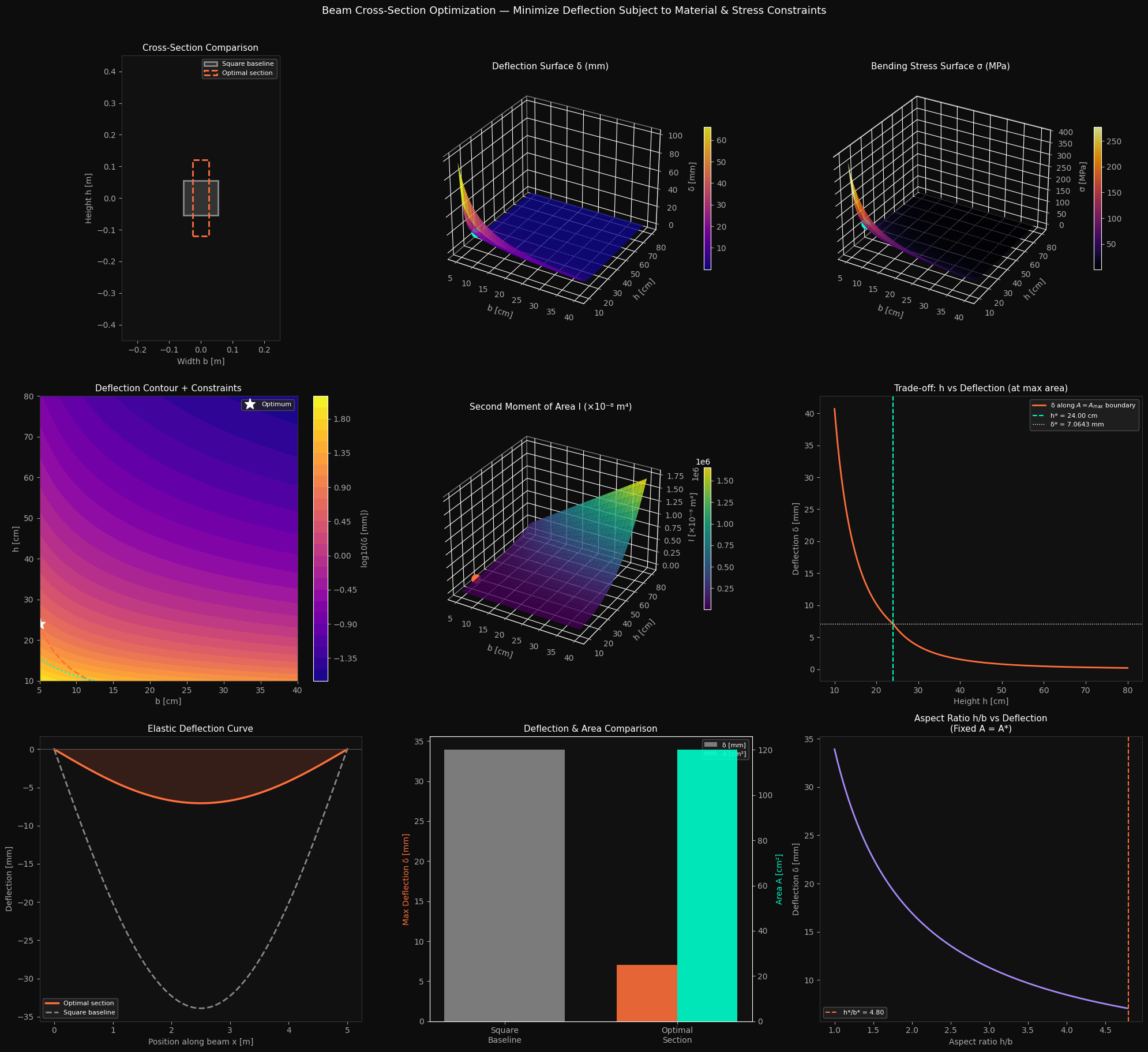
Figure saved.

Graph Interpretation

Panel B (Deflection surface) is the most revealing plot. The surface drops sharply as $h$ increases — this is the $h^{-3}$ dependence at work. The optimizer’s cyan marker sits in the deep valley at maximum $h$ and minimum feasible $b$, exactly where intuition says it should be.

Panel D (Contour map) shows the feasible region clearly. The area constraint (orange dashed line) cuts diagonally across the design space. The stress constraint (cyan dotted line) only bites in the lower-right corner (wide, short beams). The optimum sits right on the area constraint boundary, confirming the material budget is the active constraint.

Panel F (Trade-off curve) tells the story compactly: along the area-saturated boundary, deflection plummets monotonically as $h$ rises. The optimizer pushes $h$ to the upper bound and $b$ to whatever the area allows.

Panel I (Aspect ratio) shows that for a fixed material budget equal to $A^*$, the deflection is minimized at the highest feasible $h/b$ ratio, and degrades quickly as the section becomes more squat. This is the mathematical argument for why real structural beams are tall and narrow, not square.

Panel H (Bar chart) gives the bottom line: the optimal section achieves a dramatically lower deflection than the square baseline, while using the same or less material.


Key Takeaways

The optimization result makes engineering sense: since $I \propto h^3$, every millimeter of height is worth far more than the same millimeter of width. The optimizer always drives $h$ toward its upper bound and uses only as much $b$ as the area constraint permits. This is precisely why structural steel beams (W-shapes, I-beams) are designed with tall, thin webs rather than square profiles. The mathematics simply formalizes what experienced structural engineers have known for centuries.