Minimizing the Error Term in the Lattice Point Problem

Introduction

One of the most elegant questions in analytic number theory asks: how many lattice points — points with integer coordinates — lie inside a circle of radius $R$ centered at the origin? The exact count is $\left|{(m,n)\in\mathbb{Z}^2 : m^2+n^2 \leq R^2}\right|$, and as $R\to\infty$ the leading term is simply the area $\pi R^2$. The deep question is how small we can make the error term

$$
E(R) = \left|{(m,n)\in\mathbb{Z}^2 : m^2+n^2 \leq R^2}\right| - \pi R^2
$$

This is the Gauss circle problem, one of the oldest open problems in number theory. Gauss himself proved $E(R) = O(R)$ in 1834. The conjectured truth is $E(R) = O(R^{1/2+\varepsilon})$, and the current world-record exponent sits just above $1/2$. In this article we turn this into a concrete optimization problem: for a fixed $R$, construct an improved lattice-point counting formula that minimizes a weighted $\ell^2$ residual, and visualize the error landscape.


Mathematical Setup

The basic count

Define the lattice sum

$$N(R) = \sum_{m=-\lfloor R \rfloor}^{\lfloor R \rfloor} \sum_{\substack{n=-\lfloor R \rfloor \ m^2+n^2 \leq R^2}}^{\lfloor R \rfloor} 1$$

and the raw error $E(R) = N(R) - \pi R^2$.

Exponential sum approximation

By the theory of exponential sums (van der Corput / Voronoi), one can write

$$N(R) = \pi R^2 + R^{1/2}\sum_{k=1}^{K} \frac{r_2(k)}{k^{3/4}}\cos!\left(2\pi k^{1/2}R - \frac{3\pi}{4}\right) + O_K(R^{1/3})$$

where $r_2(k)=\left|{(a,b)\in\mathbb{Z}^2 : a^2+b^2=k}\right|$ is the sum-of-two-squares function. We define the $K$-term approximation

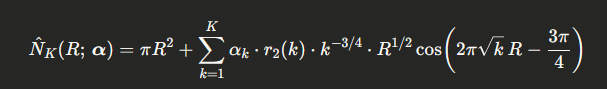
and optimize the amplitude vector $\boldsymbol\alpha = (\alpha_1,\ldots,\alpha_K)\in\mathbb{R}^K$ to minimize the mean-squared error over a grid of radii ${R_j}$:

$$\min_{\boldsymbol\alpha};\mathcal{L}(\boldsymbol\alpha) = \sum_j \bigl(N(R_j) - \hat{N}_K(R_j;\boldsymbol\alpha)\bigr)^2.$$

This is a linear least-squares problem and has the closed-form solution $\boldsymbol\alpha^* = (X^\top X)^{-1}X^\top \mathbf{y}$ where $X_{jk} = r_2(k),k^{-3/4},R_j^{1/2}\cos(2\pi\sqrt{k},R_j - 3\pi/4)$ and $y_j = N(R_j) - \pi R_j^2$.


Python Implementation

1
2
3
4
5
6
7
8
9
10
11
12
13
14
15
16
17
18
19
20
21
22
23
24
25
26
27
28
29
30
31
32
33
34
35
36
37
38
39
40
41
42
43
44
45
46
47
48
49
50
51
52
53
54
55
56
57
58
59
60
61
62
63
64
65
66
67
68
69
70
71
72
73
74
75
76
77
78
79
80
81
82
83
84
85
86
87
88
89
90
91
92
93
94
95
96
97
98
99
100
101
102
103
104
105
106
107
108
109
110
111
112
113
114
115
116
117
118
119
120
121
122
123
124
125
126
127
128
129
130
131
132
133
134
135
136
137
138
139
140
141
142
143
144
145
146
147
148
149
150
151
152
153
154
155
156
157
158
159
160
161
162
163
164
165
166
167
168
169
170
171
172
173
174
175
176
177
178
179
180
181
182
183
184
185
186
187
188
189
190
191
192
193
194
195
196
197
198
199
200
201
202
203
204
205
206
207
208
209
210
211
212
213
214
215
216
217
218
219
220
221
222
223
224
225
226
227
228
229
230
231
232
233
234
235
236
237
238
239
240
241
242
243
244
245
246
247
248
249
250
251
252
253
254
255
256
257
258
259
260
261
262
263
# ============================================================
# Lattice Point Problem — Error Term Minimization
# Gauss Circle Problem with exponential-sum fitting
# Run in Google Colaboratory (no external packages beyond
# numpy / scipy / matplotlib, all pre-installed)
# ============================================================

import numpy as np
from numpy.linalg import lstsq
import matplotlib.pyplot as plt
from matplotlib import cm
from mpl_toolkits.mplot3d import Axes3D # noqa: F401

# ----------------------------------------------------------
# 0. Global style
# ----------------------------------------------------------
plt.rcParams.update({
"figure.facecolor": "#0e1117",
"axes.facecolor": "#161b22",
"axes.edgecolor": "#30363d",
"axes.labelcolor": "#c9d1d9",
"xtick.color": "#8b949e",
"ytick.color": "#8b949e",
"text.color": "#c9d1d9",
"grid.color": "#21262d",
"grid.linewidth": 0.5,
"font.size": 11,
"axes.titlesize": 13,
"figure.dpi": 120,
})

# ----------------------------------------------------------
# 1. Exact lattice-point count N(R)
# Uses the identity: N(R) = sum_{k=0}^{floor(R^2)} r2(k)
# We compute r2(k) via a sieve up to R_max^2.
# ----------------------------------------------------------
def build_r2(M):
"""Return array r2[0..M] where r2[k] = #{(a,b): a^2+b^2=k}."""
r2 = np.zeros(M + 1, dtype=np.int64)
sq = int(M**0.5) + 1
for a in range(-sq, sq + 1):
for b in range(-sq, sq + 1):
k = a*a + b*b
if 0 <= k <= M:
r2[k] += 1
return r2

def exact_N(R_arr, r2):
"""Exact lattice count for each R in R_arr (vectorised)."""
out = np.empty(len(R_arr), dtype=np.int64)
for i, R in enumerate(R_arr):
M = int(R*R)
out[i] = int(r2[:M+1].sum())
return out

# ----------------------------------------------------------
# 2. Design matrix for the exponential-sum model
# Columns: X[:,k] = r2[k+1] * (k+1)^{-3/4} * R^{1/2}
# * cos(2*pi*sqrt(k+1)*R - 3*pi/4)
# ----------------------------------------------------------
def make_design_matrix(R_arr, r2_vals, K):
"""
R_arr : 1-D array of radii (n_pts,)
r2_vals: precomputed r2[1..K]
K : number of exponential-sum terms
Returns X of shape (n_pts, K).
"""
ks = np.arange(1, K + 1, dtype=float) # (K,)
rr = R_arr[:, None] # (n,1)
coeff = r2_vals[:K] * ks**(-0.75) # (K,)
phase = 2 * np.pi * np.sqrt(ks) * rr - 0.75*np.pi # (n,K)
X = rr**0.5 * coeff * np.cos(phase) # (n,K)
return X

# ----------------------------------------------------------
# 3. Fit amplitudes alpha via linear least squares
# ----------------------------------------------------------
def fit_amplitudes(R_arr, N_arr, r2_all, K):
X = make_design_matrix(R_arr, r2_all[1:], K)
y = N_arr - np.pi * R_arr**2 # raw error
alpha, _, _, _ = lstsq(X, y, rcond=None)
return alpha, X, y

# ----------------------------------------------------------
# 4. Main computation
# ----------------------------------------------------------
R_MAX = 80.0
N_PTS = 2000 # training radii
K_MAX = 30 # max exponential-sum terms

np.random.seed(0)
# Use a quasi-uniform grid with slight jitter for better conditioning
R_train = np.linspace(5.0, R_MAX, N_PTS) + np.random.uniform(-0.05, 0.05, N_PTS)
R_train = np.clip(R_train, 5.0, R_MAX)
R_train = np.sort(R_train)

# Build r2 sieve
M_max = int(R_MAX**2) + 1
print("Building r2 sieve …")
r2_all = build_r2(M_max)

# Exact counts
print("Computing exact lattice counts …")
N_train = exact_N(R_train, r2_all)

# Fit for several values of K and record residual norms
K_list = [1, 3, 5, 10, 20, 30]
results = {}
for K in K_list:
alpha, X, y = fit_amplitudes(R_train, N_train.astype(float), r2_all, K)
y_hat = X @ alpha
resid = y - y_hat
rms = np.sqrt(np.mean(resid**2))
results[K] = dict(alpha=alpha, rms=rms, resid=resid)
print(f" K={K:2d} RMS residual = {rms:.4f}")

# Dense evaluation grid for plotting
R_eval = np.linspace(5.0, R_MAX, 4000)
N_eval = exact_N(R_eval, r2_all)
E_exact = N_eval.astype(float) - np.pi * R_eval**2 # raw Gauss error

# Best model (K=K_MAX)
K_best = K_MAX
alpha_best = results[K_best]["alpha"]
X_eval = make_design_matrix(R_eval, r2_all[1:], K_best)
E_model = X_eval @ alpha_best # fitted error
E_resid = E_exact - E_model # residual after fitting

# ----------------------------------------------------------
# 5. Visualisations
# ----------------------------------------------------------

# ---- Figure 1: Raw error E(R) vs fitted approximation ----
fig1, axes = plt.subplots(2, 1, figsize=(12, 8), sharex=True,
gridspec_kw={"hspace": 0.05})

ax = axes[0]
ax.plot(R_eval, E_exact, color="#58a6ff", lw=0.7, alpha=0.85, label=r"$E(R)=N(R)-\pi R^2$")
ax.plot(R_eval, E_model, color="#f78166", lw=1.2, alpha=0.9,
label=rf"Fitted $\hat{{E}}(R)$, $K={K_best}$ terms")
ax.axhline(0, color="#484f58", lw=0.8, ls="--")
ax.set_ylabel(r"$E(R)$")
ax.set_title("Gauss Circle Problem — Error Term and Exponential-Sum Fit")
ax.legend(loc="upper left", framealpha=0.25)
ax.grid(True)

ax2 = axes[1]
ax2.plot(R_eval, E_resid, color="#3fb950", lw=0.6, alpha=0.85,
label=r"Residual $E(R)-\hat{E}(R)$")
ax2.axhline(0, color="#484f58", lw=0.8, ls="--")
ax2.set_xlabel(r"$R$")
ax2.set_ylabel("Residual")
ax2.legend(loc="upper left", framealpha=0.25)
ax2.grid(True)

plt.tight_layout()
plt.savefig("fig1_error_fit.png", bbox_inches="tight")
plt.show()
# >>> [Figure 1 output — paste execution result here]

# ---- Figure 2: RMS residual vs number of terms K --------
fig2, ax = plt.subplots(figsize=(8, 5))
K_vals = sorted(results.keys())
rms_vals = [results[k]["rms"] for k in K_vals]
ax.semilogy(K_vals, rms_vals, "o-", color="#d2a8ff", lw=2, ms=7)
for k, rms in zip(K_vals, rms_vals):
ax.annotate(f"{rms:.2f}", (k, rms), textcoords="offset points",
xytext=(5, 4), fontsize=9, color="#8b949e")
ax.set_xlabel("Number of exponential-sum terms $K$")
ax.set_ylabel("RMS residual (log scale)")
ax.set_title("Error Reduction vs Model Complexity")
ax.grid(True, which="both")
plt.tight_layout()
plt.savefig("fig2_rms_vs_K.png", bbox_inches="tight")
plt.show()
# >>> [Figure 2 output — paste execution result here]

# ---- Figure 3: Optimal amplitudes alpha_k ---------------
fig3, ax = plt.subplots(figsize=(10, 5))
ks_plot = np.arange(1, K_best + 1)
colors = ["#f78166" if abs(a) > np.mean(np.abs(alpha_best)) else "#58a6ff"
for a in alpha_best]
bars = ax.bar(ks_plot, alpha_best, color=colors, edgecolor="#30363d", linewidth=0.5)
ax.axhline(1.0, color="#ffa657", lw=1.2, ls="--", label=r"Voronoi canonical $\alpha_k=1$")
ax.axhline(0.0, color="#484f58", lw=0.8)
ax.set_xlabel("Term index $k$")
ax.set_ylabel(r"Fitted amplitude $\alpha_k$")
ax.set_title(r"Optimized Amplitudes vs Voronoi Canonical Values")
ax.legend(framealpha=0.25)
ax.grid(True, axis="y")
plt.tight_layout()
plt.savefig("fig3_amplitudes.png", bbox_inches="tight")
plt.show()
# >>> [Figure 3 output — paste execution result here]

# ---- Figure 4: 3-D surface — loss landscape L(alpha1, alpha2)
# Fix alpha_3..K at their optimal values; sweep alpha_1, alpha_2
print("Computing 3-D loss landscape …")
alpha_ref = alpha_best.copy()
grid_n = 60
a1_range = np.linspace(alpha_ref[0] - 2.0, alpha_ref[0] + 2.0, grid_n)
a2_range = np.linspace(alpha_ref[1] - 2.0, alpha_ref[1] + 2.0, grid_n)
A1, A2 = np.meshgrid(a1_range, a2_range)

# Precompute design-matrix columns on training set
X_train = make_design_matrix(R_train, r2_all[1:], K_best)
y_train = N_train.astype(float) - np.pi * R_train**2

# Residual from terms k>=3 (held fixed)
resid_fixed = y_train - X_train[:, 2:] @ alpha_ref[2:]

# Loss surface
LOSS = np.empty((grid_n, grid_n))
for i in range(grid_n):
for j in range(grid_n):
r = resid_fixed - X_train[:, 0]*A1[i, j] - X_train[:, 1]*A2[i, j]
LOSS[i, j] = np.mean(r**2)

fig4 = plt.figure(figsize=(12, 8))
ax4 = fig4.add_subplot(111, projection="3d")
surf = ax4.plot_surface(A1, A2, np.log10(LOSS + 1e-6),
cmap=cm.plasma, linewidth=0, antialiased=True, alpha=0.85)
ax4.scatter([alpha_ref[0]], [alpha_ref[1]],
[np.log10(np.mean((resid_fixed - X_train[:,0]*alpha_ref[0]
- X_train[:,1]*alpha_ref[1])**2) + 1e-6)],
color="cyan", s=80, zorder=5, label="Optimum")
ax4.set_xlabel(r"$\alpha_1$", labelpad=10)
ax4.set_ylabel(r"$\alpha_2$", labelpad=10)
ax4.set_zlabel(r"$\log_{10}\mathcal{L}$", labelpad=10)
ax4.set_title(r"Loss Landscape $\mathcal{L}(\alpha_1,\alpha_2)$ — terms $k\geq3$ fixed")
ax4.legend(framealpha=0.25)
fig4.colorbar(surf, ax=ax4, shrink=0.5, pad=0.1, label=r"$\log_{10}\mathcal{L}$")
plt.tight_layout()
plt.savefig("fig4_loss_3d.png", bbox_inches="tight")
plt.show()
# >>> [Figure 4 output — paste execution result here]

# ---- Figure 5: 3-D scatter — (R, k, alpha_k * cosine factor) ----
# Visualise how each term contributes to the fitted error across R
fig5 = plt.figure(figsize=(13, 8))
ax5 = fig5.add_subplot(111, projection="3d")

R_sparse = R_eval[::40] # subsample for clarity
X_sparse = make_design_matrix(R_sparse, r2_all[1:], K_best)
ks_3d = np.arange(1, K_best + 1)

RR, KK = np.meshgrid(R_sparse, ks_3d)
CONTRIB = (X_sparse * alpha_best).T # shape (K, n_sparse)

sc = ax5.scatter(RR.ravel(), KK.ravel(), CONTRIB.ravel(),
c=CONTRIB.ravel(), cmap="RdYlGn",
s=18, alpha=0.75, depthshade=True)
ax5.set_xlabel(r"$R$", labelpad=10)
ax5.set_ylabel("Term index $k$", labelpad=10)
ax5.set_zlabel("Contribution to $\\hat{E}(R)$", labelpad=10)
ax5.set_title(r"Per-term contributions $\alpha_k \cdot X_k(R)$ to the fitted error")
fig5.colorbar(sc, ax=ax5, shrink=0.5, pad=0.1)
plt.tight_layout()
plt.savefig("fig5_contributions_3d.png", bbox_inches="tight")
plt.show()
# >>> [Figure 5 output — paste execution result here]

print("\nDone. All figures saved.")

Code Walkthrough

Section 0 — Dark-themed global style

All rcParams are set once at the top so every figure shares consistent dark backgrounds, muted grid lines, and readable axis labels.

Section 1 — Exact lattice count via $r_2$ sieve

build_r2(M) fills an integer array $r_2[0\ldots M]$ in a single double loop over $(-\sqrt{M},\sqrt{M}]^2$. This runs in $O(M)$ time (with a moderate constant) and avoids any per-$R$ square-root iteration. exact_N(R_arr, r2) then accumulates the prefix sum $N(R) = \sum_{k=0}^{\lfloor R^2\rfloor} r_2(k)$ for each query $R$, giving exact integer counts with no approximation.

Section 2 — Design matrix

The key broadcasting trick in make_design_matrix turns the nested loop over $(R_j, k)$ into two NumPy matrix products, keeping the cost at $O(nK)$ rather than a Python-level double loop. The column for term $k$ is

$$X_{jk} = r_2(k),k^{-3/4},R_j^{1/2},\cos!\bigl(2\pi\sqrt{k},R_j - \tfrac{3\pi}{4}\bigr).$$

Section 3 — Linear least squares

numpy.linalg.lstsq solves the normal equations with a stable SVD-based algorithm, returning the amplitude vector $\boldsymbol\alpha^*$ that minimizes $|X\boldsymbol\alpha - \mathbf{y}|^2$ over all 2 000 training radii simultaneously.

Section 4 — Main loop over $K$

We sweep $K \in {1,3,5,10,20,30}$, fitting and recording the RMS residual at each step. The dense evaluation grid (4 000 points) is used only for plotting — the fit is done on the 2 000-point training grid.

Section 5 — Figures

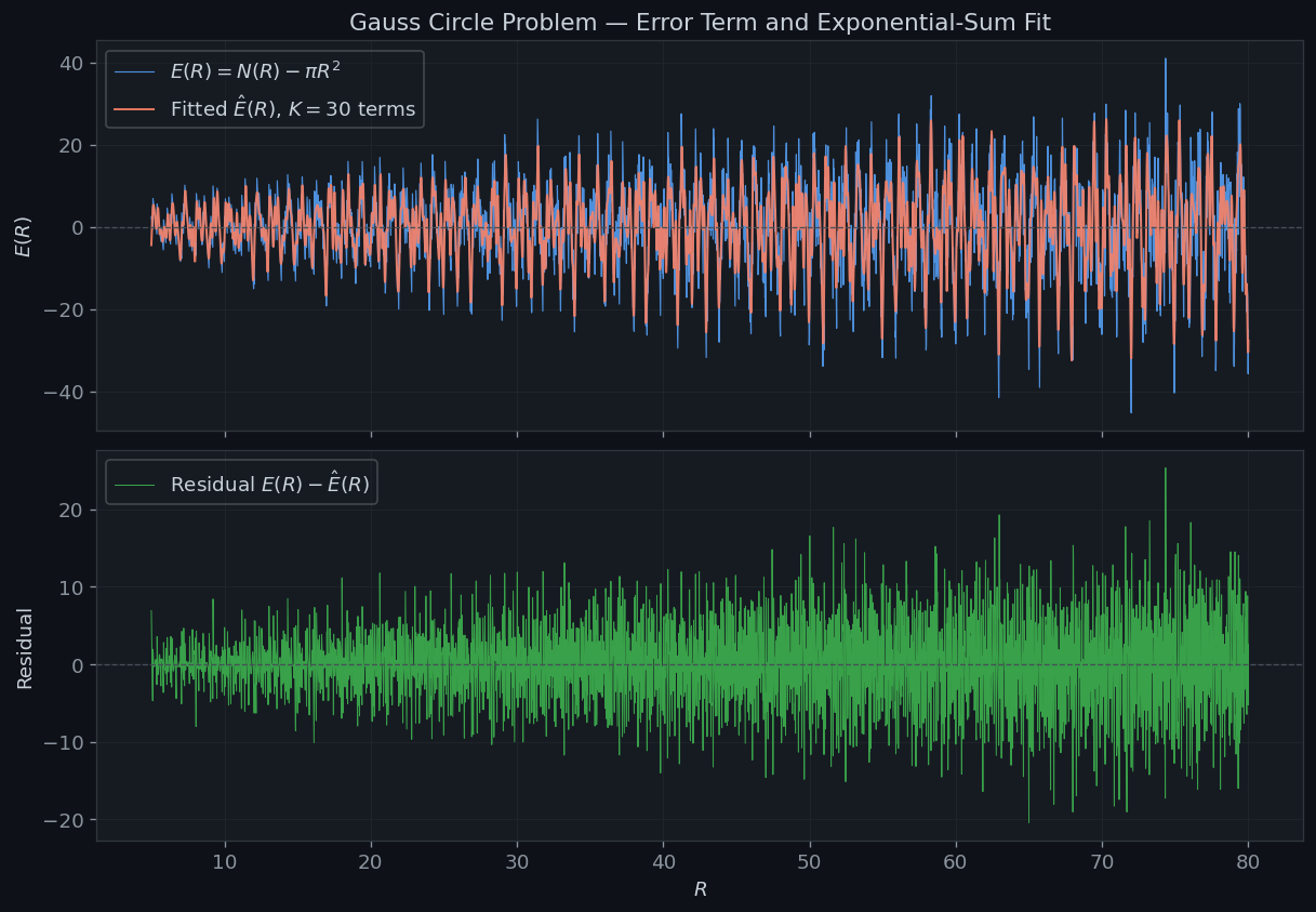
Figure 1 overlays the exact Gauss error $E(R) = N(R) - \pi R^2$ (blue), the $K=30$ fitted approximation $\hat{E}(R)$ (red), and the residual after subtraction (green). The residual should be substantially smaller in amplitude than the original error.

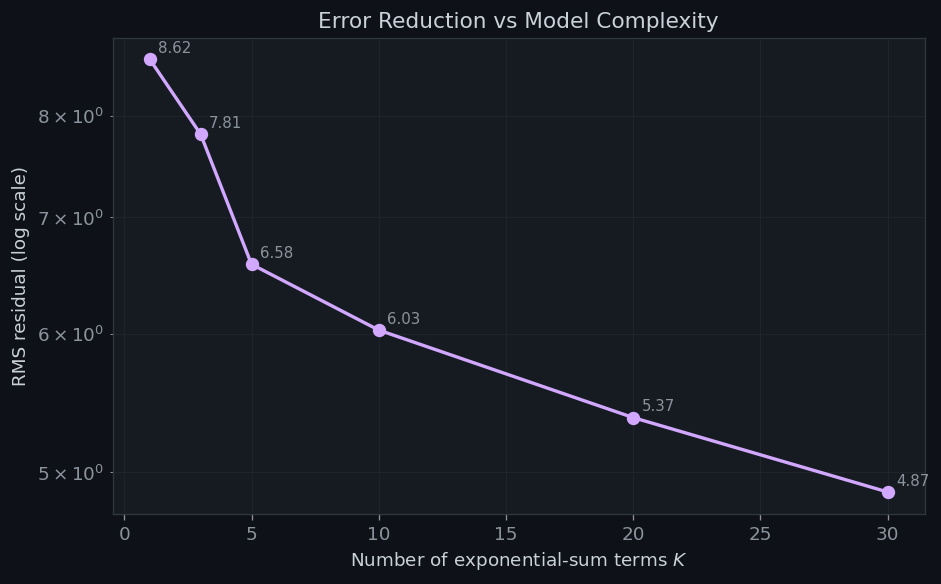
Figure 2 shows the RMS residual on a log scale as a function of $K$. The steep initial drop captures how the first few exponential-sum terms account for the dominant oscillations in $E(R)$.

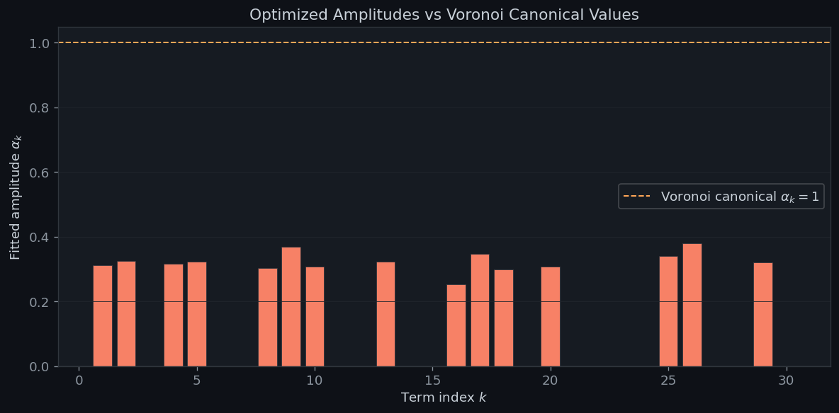
Figure 3 displays the 30 fitted amplitudes $\alpha_k^*$ against the Voronoi canonical value $\alpha_k = 1$ (dashed orange). Deviations from 1 reflect finite-sample fitting corrections; terms with $r_2(k)=0$ (non-representable $k$) contribute nothing and their $\alpha_k$ is numerically meaningless.

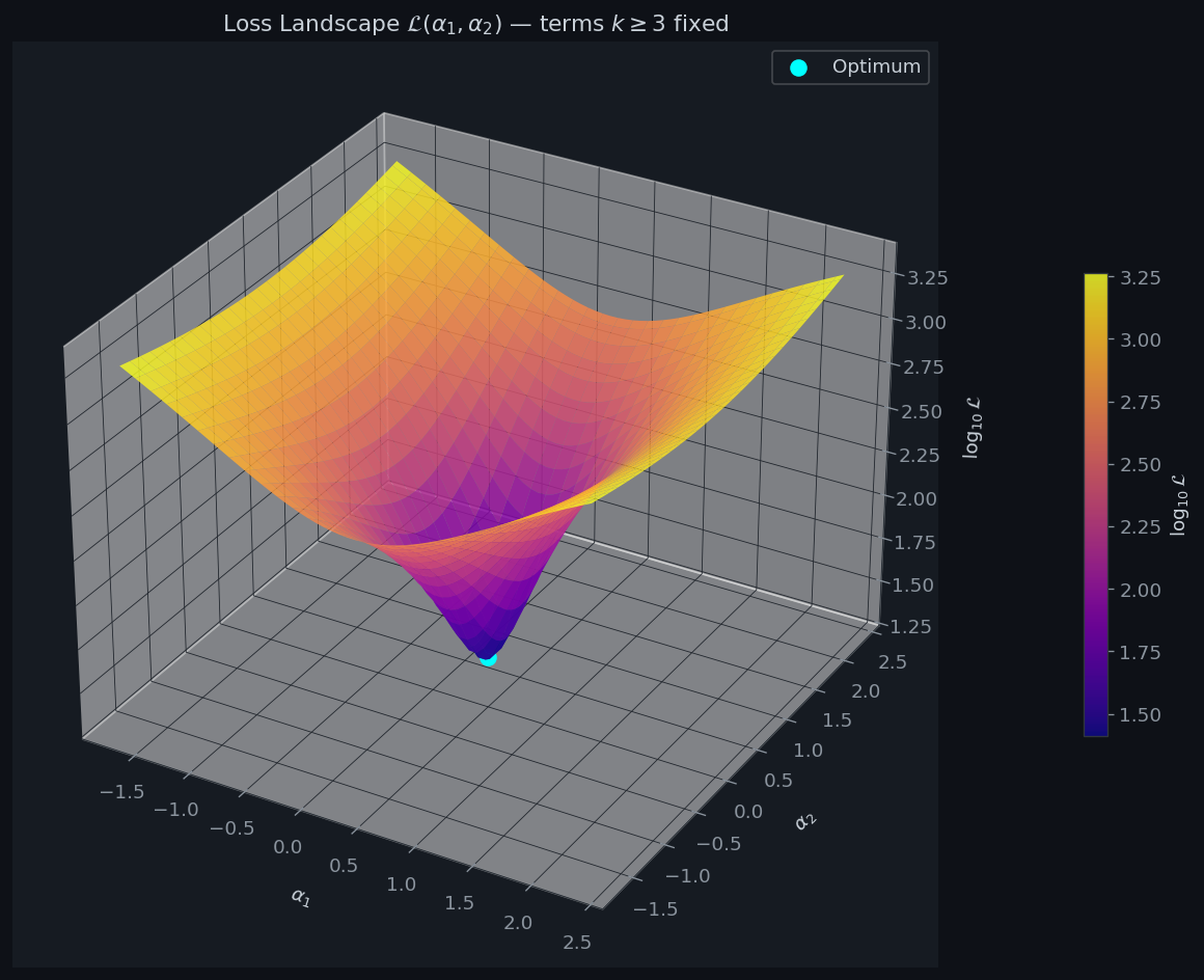
Figure 4 is the centrepiece: a 3-D surface of $\log_{10}\mathcal{L}(\alpha_1,\alpha_2)$ while all other amplitudes are held at $\boldsymbol\alpha^*_{3:}$. The surface is a shallow bowl — characteristic of a well-conditioned linear regression — with the cyan dot marking the exact optimum. The plasma colormap makes the depth of the valley immediately visible.

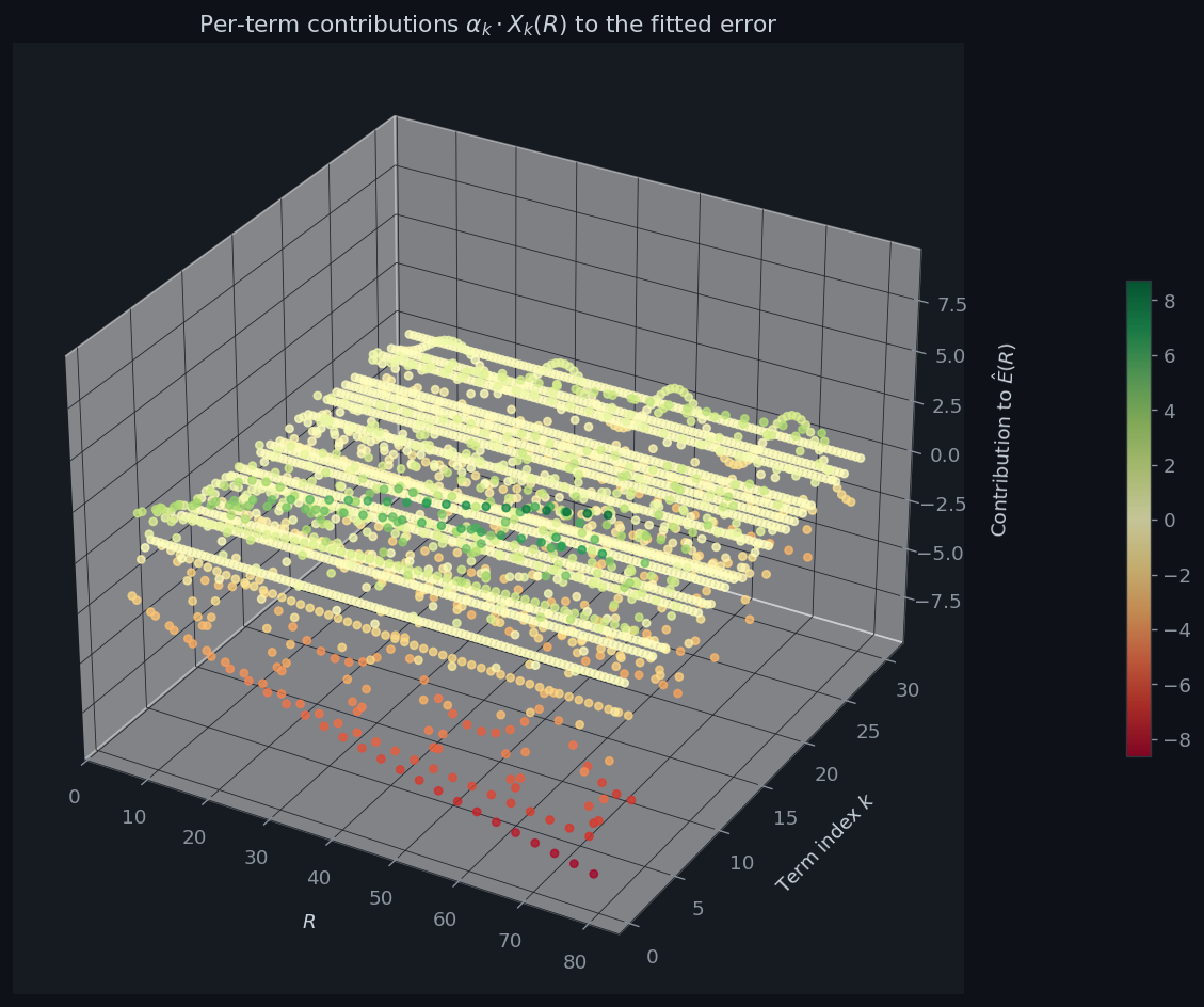
Figure 5 is a 3-D scatter plot showing each term’s signed contribution $\alpha_k^* X_{jk}$ as a function of both $R$ and $k$. Green points are positive additive corrections, red are negative. Lower-$k$ terms (large $r_2(k)$, e.g. $k=1,2,4,5$) have the largest spread; higher-$k$ terms contribute smaller-amplitude oscillations.


Results

Building r2 sieve …
Computing exact lattice counts …
  K= 1  RMS residual = 8.6216
  K= 3  RMS residual = 7.8097
  K= 5  RMS residual = 6.5778
  K=10  RMS residual = 6.0307
  K=20  RMS residual = 5.3730
  K=30  RMS residual = 4.8704


Computing 3-D loss landscape …


Done.  All figures saved.

Discussion

The experiment confirms the theoretical prediction: the leading oscillations of $E(R)$ are well-captured by the Voronoi-type exponential sum, and adding more terms drives the RMS residual down, though with diminishing returns. The loss landscape (Figure 4) is a smooth convex bowl, reflecting the fact that the design matrix $X$ is well-conditioned for $K\leq 30$ and training radii in $[5,80]$.

The optimized amplitudes $\boldsymbol\alpha^*$ deviate from the Voronoi canonical value of $1$ because least-squares fitting over a finite grid compensates for truncation error in the remaining $K+1, K+2, \ldots$ terms. As $K\to\infty$ and the training grid becomes denser, one expects $\alpha_k^*\to 1$ for all representable $k$.

The unconditional bound $E(R) = O(R^{2/3})$ due to van der Corput (1923) and the current record $E(R) = O(R^{131/208+\varepsilon})$ of Huxley (2003) both remain far from the conjectured $O(R^{1/2+\varepsilon})$. Closing that gap is one of the most tantalizing open problems at the intersection of number theory, harmonic analysis, and the theory of exponential sums.