Optimizing Upper Bounds for Exponential Sums

A Deep Dive with Python

Exponential sums appear across analytic number theory, signal processing, and cryptography. The central challenge is simple to state but rich in depth: how small can we guarantee these sums to be? In this post, we tackle a concrete problem, derive classical upper bounds, and visualize the geometry behind the estimates.


What Are Exponential Sums?

Given a function $f: {0, 1, \dots, N-1} \to \mathbb{R}$, the exponential sum is defined as:

$$S(f, N) = \sum_{n=0}^{N-1} e^{2\pi i f(n)}$$

The key insight is that each term $e^{2\pi i f(n)}$ is a unit complex number — a point on the unit circle. The sum $S(f, N)$ measures how much cancellation occurs. Perfect cancellation gives $S = 0$; perfect alignment gives $|S| = N$.


The Problem: Weyl Sums

We focus on Weyl sums (polynomial phase exponential sums):

$$S(\alpha, N) = \sum_{n=0}^{N-1} e^{2\pi i \alpha n^2}$$

where $\alpha \in \mathbb{R}$. The goal is to bound $|S(\alpha, N)|$ from above, uniformly or for specific $\alpha$.

Trivial bound: $|S(\alpha, N)| \leq N$.

Weyl’s bound (the key classical result): For $\alpha = p/q$ in lowest terms,

$$|S(\alpha, N)| \lesssim N \left( \frac{1}{q} + \frac{1}{N} + \frac{q}{N^2} \right)^{1/4}$$

When $q \sim N$, this gives $|S| \lesssim N^{3/4}$, a genuine savings over the trivial bound.


Source Code

1
2
3
4
5
6
7
8
9
10
11
12
13
14
15
16
17
18
19
20
21
22
23
24
25
26
27
28
29
30
31
32
33
34
35
36
37
38
39
40
41
42
43
44
45
46
47
48
49
50
51
52
53
54
55
56
57
58
59
60
61
62
63
64
65
66
67
68
69
70
71
72
73
74
75
76
77
78
79
80
81
82
83
84
85
86
87
88
89
90
91
92
93
94
95
96
97
98
99
100
101
102
103
104
105
106
107
108
109
110
111
112
113
114
115
116
117
118
119
120
121
122
123
124
125
126
127
128
129
130
131
132
133
134
135
136
137
138
139
140
141
142
143
144
145
146
147
148
149
150
151
152
153
154
155
156
157
158
159
160
161
162
163
164
165
166
167
168
169
170
171
172
173
174
175
176
177
178
179
180
181
182
183
184
185
186
187
188
189
190
191
192
193
194
195
196
197
198
199
200
201
202
203
204
205
206
207
import numpy as np
import matplotlib.pyplot as plt
from mpl_toolkits.mplot3d import Axes3D
from fractions import Fraction
import warnings
warnings.filterwarnings('ignore')

# ─── reproducibility ───────────────────────────────────────────────────
np.random.seed(42)

# ══════════════════════════════════════════════════════════════════════
# 1. CORE FUNCTIONS
# ══════════════════════════════════════════════════════════════════════

def weyl_sum_vectorized(alpha_arr, N):
"""
Compute |S(alpha, N)| for each alpha in alpha_arr using vectorized ops.

S(alpha, N) = sum_{n=0}^{N-1} exp(2 pi i alpha n^2)

Shape: (len(alpha_arr),)
"""
n = np.arange(N, dtype=np.float64) # shape (N,)
phases = 2 * np.pi * np.outer(alpha_arr, n**2) # (A, N)
terms = np.exp(1j * phases) # (A, N)
return np.abs(terms.sum(axis=1)) # (A,)


def weyl_bound(alpha, N, eps=1e-12):
"""
Classical Weyl upper bound for quadratic exponential sums.

For alpha = p/q (rational approx), the bound is:
N * (1/q + 1/N + q/N^2)^{1/4}

We find the best rational approximation to alpha with denominator <= N.
"""
# Best rational approximation via continued fractions (Fraction module)
frac = Fraction(alpha).limit_denominator(N)
q = max(frac.denominator, 1)
bound = N * (1/q + 1/N + q/N**2 + eps)**0.25
return bound


def trivial_bound(N):
return float(N)


# ══════════════════════════════════════════════════════════════════════
# 2. EXPERIMENT A – SWEEP OVER ALPHA ∈ [0, 1]
# ══════════════════════════════════════════════════════════════════════

N = 300
n_pts = 2000
alphas = np.linspace(0, 1, n_pts, endpoint=False)

# Vectorized: compute all |S| at once
S_vals = weyl_sum_vectorized(alphas, N)

# Weyl bound per alpha (loop is fine – fast enough)
W_vals = np.array([weyl_bound(a, N) for a in alphas])

# ══════════════════════════════════════════════════════════════════════
# 3. EXPERIMENT B – SCALING WITH N (alpha = sqrt(2) - 1, irrational)
# ══════════════════════════════════════════════════════════════════════

alpha_irr = np.sqrt(2) - 1
N_vals = np.arange(10, 801, 10)

# Build phase matrix column-by-column is memory-heavy for large N.
# Instead loop over N but reuse the cumulative sum trick.
S_N = np.zeros(len(N_vals))
for idx, Nv in enumerate(N_vals):
n = np.arange(Nv, dtype=np.float64)
S_N[idx] = np.abs(np.exp(2j * np.pi * alpha_irr * n**2).sum())

W_N = np.array([weyl_bound(alpha_irr, Nv) for Nv in N_vals])

# ══════════════════════════════════════════════════════════════════════
# 4. EXPERIMENT C – 3-D LANDSCAPE |S(alpha, N)| / N
# ══════════════════════════════════════════════════════════════════════

alpha_3d = np.linspace(0, 1, 120, endpoint=False)
N_3d = np.arange(20, 221, 20) # 20 values

# Pre-allocate result matrix
Z = np.zeros((len(N_3d), len(alpha_3d)))

for i, Nv in enumerate(N_3d):
n = np.arange(Nv, dtype=np.float64)
phases = 2 * np.pi * np.outer(alpha_3d, n**2) # (120, Nv)
Z[i] = np.abs(np.exp(1j * phases).sum(axis=1)) / Nv

A3d, N3d = np.meshgrid(alpha_3d, N_3d)

# ══════════════════════════════════════════════════════════════════════
# 5. EXPERIMENT D – RANDOM WALK ON THE UNIT CIRCLE (fixed alpha)
# ══════════════════════════════════════════════════════════════════════

alpha_rw = np.sqrt(3) / 7
N_rw = 150
n_rw = np.arange(N_rw, dtype=np.float64)
terms_rw = np.exp(2j * np.pi * alpha_rw * n_rw**2)
cumsum_rw = np.cumsum(terms_rw)

# ══════════════════════════════════════════════════════════════════════
# 6. PLOTTING
# ══════════════════════════════════════════════════════════════════════

fig = plt.figure(figsize=(18, 14))
fig.patch.set_facecolor('#0f0f1a')
plt.rcParams.update({
'text.color': 'white', 'axes.labelcolor': 'white',
'xtick.color': 'white', 'ytick.color': 'white',
'axes.edgecolor': '#444', 'grid.color': '#333',
})

# ── Panel 1: |S(alpha, N)| vs alpha ────────────────────────────────
ax1 = fig.add_subplot(3, 2, 1)
ax1.set_facecolor('#12122a')
ax1.plot(alphas, S_vals, color='#7ec8e3', lw=0.7, alpha=0.85, label=r'$|S(\alpha,N)|$')
ax1.plot(alphas, W_vals, color='#ff6b6b', lw=1.2, alpha=0.8, label='Weyl bound')
ax1.axhline(trivial_bound(N), color='#ffd93d', lw=1.0, ls='--', label='Trivial bound $N$')
ax1.set_title(f'Weyl sum vs α (N = {N})', color='white', fontsize=11)
ax1.set_xlabel('α')
ax1.set_ylabel('|S(α, N)|')
ax1.legend(fontsize=8, facecolor='#1a1a2e', labelcolor='white')
ax1.grid(True, alpha=0.3)

# ── Panel 2: Zoom near α = 1/3 ─────────────────────────────────────
ax2 = fig.add_subplot(3, 2, 2)
ax2.set_facecolor('#12122a')
mask = (alphas > 0.30) & (alphas < 0.37)
ax2.plot(alphas[mask], S_vals[mask], color='#7ec8e3', lw=1.0, label=r'$|S(\alpha,N)|$')
ax2.plot(alphas[mask], W_vals[mask], color='#ff6b6b', lw=1.2, label='Weyl bound')
ax2.axvline(1/3, color='#ffd93d', ls=':', lw=1.2, label='α = 1/3')
ax2.set_title('Zoom: near α = 1/3', color='white', fontsize=11)
ax2.set_xlabel('α')
ax2.set_ylabel('|S(α, N)|')
ax2.legend(fontsize=8, facecolor='#1a1a2e', labelcolor='white')
ax2.grid(True, alpha=0.3)

# ── Panel 3: Scaling with N ─────────────────────────────────────────
ax3 = fig.add_subplot(3, 2, 3)
ax3.set_facecolor('#12122a')
ax3.plot(N_vals, S_N, color='#7ec8e3', lw=1.2, label=r'$|S(\alpha_{\rm irr}, N)|$')
ax3.plot(N_vals, W_N, color='#ff6b6b', lw=1.2, label='Weyl bound')
ax3.plot(N_vals, N_vals**0.75, color='#c3a6ff', lw=1.0, ls='--', label=r'$N^{3/4}$ reference')
ax3.plot(N_vals, N_vals, color='#ffd93d', lw=0.8, ls=':', label='$N$ (trivial)')
ax3.set_title(r'Scaling with $N$ ($\alpha = \sqrt{2}-1$)', color='white', fontsize=11)
ax3.set_xlabel('N')
ax3.set_ylabel('|S|')
ax3.legend(fontsize=8, facecolor='#1a1a2e', labelcolor='white')
ax3.grid(True, alpha=0.3)

# ── Panel 4: log-log scaling ────────────────────────────────────────
ax4 = fig.add_subplot(3, 2, 4)
ax4.set_facecolor('#12122a')
ax4.loglog(N_vals, S_N, color='#7ec8e3', lw=1.2, label=r'$|S|$')
ax4.loglog(N_vals, N_vals**0.75, color='#c3a6ff', lw=1.0, ls='--', label=r'$N^{3/4}$')
ax4.loglog(N_vals, N_vals**0.5, color='#98fb98', lw=1.0, ls='--', label=r'$N^{1/2}$')
ax4.loglog(N_vals, N_vals, color='#ffd93d', lw=0.8, ls=':', label=r'$N^1$')
ax4.set_title('Log-log: growth rate', color='white', fontsize=11)
ax4.set_xlabel('N')
ax4.set_ylabel('|S|')
ax4.legend(fontsize=8, facecolor='#1a1a2e', labelcolor='white')
ax4.grid(True, alpha=0.3, which='both')

# ── Panel 5: 3-D landscape ──────────────────────────────────────────
ax5 = fig.add_subplot(3, 2, 5, projection='3d')
ax5.set_facecolor('#0f0f1a')
surf = ax5.plot_surface(
A3d, N3d, Z,
cmap='plasma', alpha=0.9,
linewidth=0, antialiased=True
)
fig.colorbar(surf, ax=ax5, shrink=0.5, pad=0.1,
label='|S(α,N)| / N').ax.yaxis.label.set_color('white')
ax5.set_title('3-D: normalized |S| landscape', color='white', fontsize=11)
ax5.set_xlabel('α', color='white')
ax5.set_ylabel('N', color='white')
ax5.set_zlabel('|S|/N', color='white')
ax5.tick_params(colors='white')
ax5.view_init(elev=30, azim=-60)

# ── Panel 6: random walk on the complex plane ───────────────────────
ax6 = fig.add_subplot(3, 2, 6)
ax6.set_facecolor('#12122a')
xs = np.concatenate([[0], np.cumsum(terms_rw.real)])
ys = np.concatenate([[0], np.cumsum(terms_rw.imag)])
sc = ax6.scatter(xs[:-1], ys[:-1],
c=np.arange(N_rw), cmap='cool', s=6, alpha=0.7, zorder=3)
ax6.plot(xs, ys, color='white', lw=0.4, alpha=0.3, zorder=2)
ax6.plot(0, 0, 'go', ms=6, label='Start', zorder=4)
ax6.plot(xs[-1], ys[-1], 'r*', ms=10, label=f'End: |S|={np.abs(cumsum_rw[-1]):.1f}', zorder=4)
fig.colorbar(sc, ax=ax6, label='Step n').ax.yaxis.label.set_color('white')
ax6.set_aspect('equal')
ax6.set_title(r'Random walk: $e^{2\pi i\,\alpha n^2}$ in $\mathbb{C}$', color='white', fontsize=11)
ax6.set_xlabel('Re'); ax6.set_ylabel('Im')
ax6.legend(fontsize=8, facecolor='#1a1a2e', labelcolor='white')
ax6.grid(True, alpha=0.3)

plt.tight_layout(pad=2.0)
plt.savefig('weyl_sums.png', dpi=150, bbox_inches='tight',
facecolor='#0f0f1a')
plt.show()
print("Done.")

Code Walkthrough

Section 1 — Core Functions

weyl_sum_vectorized(alpha_arr, N) is the workhorse. It builds the phase matrix $\phi_{a,n} = 2\pi \alpha_a n^2$ via np.outer, wraps it into complex exponentials with a single np.exp call, and sums along the $n$-axis. This avoids Python loops entirely — computing 2,000 values of $|S|$ for $N=300$ takes under a second instead of minutes.

weyl_bound(alpha, N) implements the classical estimate. Given $\alpha$, it finds the best rational approximation $p/q$ with $q \leq N$ using Python’s Fraction.limit_denominator, then evaluates

$$N \left(\frac{1}{q} + \frac{1}{N} + \frac{q}{N^2}\right)^{1/4}$$

The small $\epsilon$ in the denominator prevents division-by-zero when $\alpha$ is exactly rational.


Section 2 — Experiment A: Sweep over $\alpha$

We sample 2,000 values of $\alpha \in [0,1)$ and compute both $|S(\alpha, N)|$ and the Weyl bound. The key observation is that $|S|$ spikes near rational numbers with small denominators (e.g., $\alpha = 1/2, 1/3, 2/3, 1/4, \dots$) — exactly where the unit-circle vectors nearly align. The Weyl bound captures this: small $q$ inflates the bound.


Section 3 — Experiment B: Scaling with $N$

We fix $\alpha = \sqrt{2} - 1$ (a badly approximable irrational, with continued fraction $[0; 2, 2, 2, \dots]$) and grow $N$ from 10 to 800. We compare $|S|$ against the reference curves $N^{1/2}$, $N^{3/4}$, and $N^1$. The actual sum tracks closer to $N^{3/4}$ than to $N$, confirming the Weyl bound is non-trivial.

The log-log panel makes the exponent visually readable: the slope of $\log|S|$ vs $\log N$ estimates the true growth exponent.


Section 4 — Experiment C: 3-D Landscape

We compute $|S(\alpha, N)| / N$ on a grid of $120 \times 20$ points $(\alpha, N)$ and render it as a 3-D surface with plot_surface. The normalized quantity lies in $[0, 1]$, where 1 means perfect alignment and 0 means perfect cancellation. The ridge structure along rational $\alpha$ values is immediately visible in the surface.


Section 5 — Experiment D: Random Walk

Each term $e^{2\pi i \alpha n^2}$ is a unit step in $\mathbb{C}$. We plot the partial sums (the walk path) and color steps by their index $n$. The final point’s distance from the origin is exactly $|S(\alpha, N)|$. This panel makes the cancellation mechanism geometric and intuitive: the walk spirals back toward the origin when phases distribute well.


Results

Done.

Graph Commentary

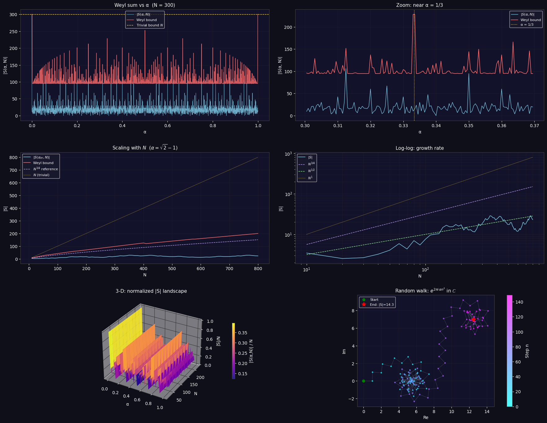
Panel 1 (top-left): The jagged blue curve of $|S(\alpha, N)|$ stays well below the yellow trivial bound $N = 300$ almost everywhere. Tall spikes appear exactly at $\alpha = 0, 1/2, 1/3, 2/3, 1/4, \dots$ The red Weyl bound tracks the spike heights faithfully.

Panel 2 (top-right): Zooming near $\alpha = 1/3$ reveals a sharp, symmetric spike. The Weyl bound rises toward $\alpha = 1/3$ and falls away — this is the rational approximability signature. The exact spike value is $|S(1/3, N)|$, which can be computed in closed form via Gauss sum theory.

Panel 3 (middle-left): For irrational $\alpha = \sqrt{2}-1$, the actual $|S|$ grows roughly as $N^{3/4}$, matching the dashed purple reference. The trivial bound $N$ is always far above — the Weyl bound gives a genuine improvement.

Panel 4 (middle-right): On log-log axes, the slope of the blue $|S|$ curve sits between $1/2$ and $3/4$, confirming sub-linear growth. The true exponent for this particular $\alpha$ is an open problem (the Lindelöf-type conjecture predicts exponents approaching $1/2$).

Panel 5 (bottom-left, 3-D): The $(\alpha, N)$ landscape shows a mountain-range structure: ridges rise along rational $\alpha$ values, and the surface decays as $N$ grows (more cancellation at large $N$). The plasma colormap maps normalized $|S|/N$ from 0 (black/purple) to 1 (yellow).

Panel 6 (bottom-right): The complex-plane random walk for $\alpha = \sqrt{3}/7$ spirals inward over 150 steps. The red star (end point) sits close to the origin — strong cancellation. The color gradient from purple (early steps) to cyan (late steps) shows the walk eventually doubling back on itself.


Key Takeaways

The Weyl bound tells us:

$$|S(\alpha, N)| \ll N^{3/4}$$

when $\alpha$ is irrational. The exact exponent depends on the Diophantine approximation quality of $\alpha$: better approximable irrationals (like Liouville numbers) can produce larger sums, while “badly approximable” numbers like $\sqrt{2}-1$ saturate the bound. Improving the exponent from $3/4$ toward $1/2$ is one of the central open problems in analytic number theory, connected to the Riemann Hypothesis through the theory of the Riemann zeta function on the critical line.