Optimizing the Selberg Sieve Weight Function

A Computational Exploration

The Selberg sieve is one of the most powerful tools in analytic number theory, producing sharper upper bounds on prime-counting problems than the classical Legendre or Brun sieves. At its heart lies a variational problem: choose a sequence of real weights $\lambda_d$ to minimize an upper bound on the number of integers in a set that avoid all small prime factors. This post walks through a concrete optimization example, solves it numerically, and visualizes the weight landscape in 2D and 3D.

---

The Mathematical Setup

Let $\mathcal{A} = {1, 2, \ldots, N}$ and let $\mathcal{P}$ be the set of primes up to $z$. The Selberg sieve produces the upper bound

$$S(\mathcal{A}, \mathcal{P}, z) \leq \sum_{n \leq N} \left(\sum_{\substack{d \mid n \ d \mid P(z)}} \lambda_d\right)^2$$

where $P(z) = \prod_{p \leq z} p$, and the weights satisfy $\lambda_1 = 1$ and $\lambda_d = 0$ for $d > z$.

Expanding the square and swapping the order of summation, this equals

$$\sum_{d_1, d_2} \lambda_{d_1} \lambda_{d_2} \cdot \left\lfloor \frac{N}{[d_1, d_2]} \right\rfloor$$

Approximating $\lfloor N / [d_1, d_2] \rfloor \approx N / [d_1, d_2]$ and using the identity $[d_1, d_2] = d_1 d_2 / \gcd(d_1, d_2)$, the bound becomes

$$N \sum_{d_1, d_2} \frac{\lambda_{d_1} \lambda_{d_2} \gcd(d_1, d_2)}{d_1 d_2}$$

The Selberg optimization problem is therefore:

$$\min_ \quad Q(\lambda) = \sum_{d_1, d_2 \mid P(z)} \frac{\lambda_{d_1} \lambda_{d_2} \gcd(d_1, d_2)}{d_1 d_2} \quad \text{subject to} \quad \lambda_1 = 1$$

This is a constrained quadratic optimization in the variables $\lambda_d$ for square-free $d \mid P(z)$ with $d \leq z$.

---

Concrete Example: Primes up to $z = 30$, $N = 10^5$

We take the sieving limit $z = 30$, so the relevant primes are ${2, 3, 5, 7, 11, 13, 17, 19, 23, 29}$ and the square-free divisors of $P(30)$ that are at most $30$ form the index set. The matrix $M_{d_1 d_2} = \gcd(d_1, d_2)/(d_1 d_2)$ is symmetric and positive definite, so the constrained quadratic problem has a unique global minimum.

The optimal weights admit the Selberg closed form:

$$\lambda_d = \mu(d) \cdot \frac{\phi(d)^{-1}}{\sum_{e \leq z} \mu(e)^2 / \phi(e)}$$

but we solve it numerically via scipy.optimize and also compute the analytic solution, then compare.

---

Python Source Code

import numpy as np
from math import gcd
from itertools import combinations
from functools import reduce
import scipy.optimize as opt
import matplotlib.pyplot as plt
from mpl_toolkits.mplot3d import Axes3D
from matplotlib import cm
import warnings
warnings.filterwarnings("ignore")

plt.style.use("dark_background")

# ── helpers ──────────────────────────────────────────────────────────────────

def primes_up_to(z):
    sieve = list(range(2, z + 1))
    for i in range(len(sieve)):
        if sieve[i]:
            p = sieve[i]
            for j in range(i + p, len(sieve), p):
                sieve[j] = 0
    return [x for x in sieve if x]

def mobius(n):
    """Möbius function μ(n)."""
    if n == 1:
        return 1
    factors = []
    temp = n
    for p in range(2, int(temp**0.5) + 1):
        if temp % p == 0:
            factors.append(p)
            temp //= p
            if temp % p == 0:
                return 0   # squared factor
    if temp > 1:
        factors.append(temp)
    return (-1) ** len(factors)

def euler_phi(n):
    """Euler's totient φ(n)."""
    result = n
    temp = n
    for p in range(2, int(temp**0.5) + 1):
        if temp % p == 0:
            while temp % p == 0:
                temp //= p
            result -= result // p
    if temp > 1:
        result -= result // temp
    return result

def squarefree_divisors(primes):
    """All square-free products of subsets of primes (including 1)."""
    divs = [1]
    for p in primes:
        divs += [d * p for d in divs]
    return sorted(divs)

# ── problem setup ─────────────────────────────────────────────────────────────

z = 30
N = 100_000
P_primes = primes_up_to(z)
print(f"Primes up to z={z}: {P_primes}")

# Index set: square-free divisors of P(z) that are <= z
all_sqfree = squarefree_divisors(P_primes)
D = [d for d in all_sqfree if d <= z]
print(f"Number of divisors in index set: {len(D)}")
print(f"Divisors: {D}")

n = len(D)
idx = {d: i for i, d in enumerate(D)}

# ── build the Gram matrix M ──────────────────────────────────────────────────

M = np.zeros((n, n))
for i, d1 in enumerate(D):
    for j, d2 in enumerate(D):
        g = gcd(d1, d2)
        M[i, j] = g / (d1 * d2)

print(f"\nGram matrix M shape: {M.shape}")
print(f"M is symmetric: {np.allclose(M, M.T)}")
print(f"Min eigenvalue of M: {np.linalg.eigvalsh(M).min():.6e}  (positive ← PD)")

# ── numerical optimization ───────────────────────────────────────────────────

# Objective: lambda^T M lambda  (quadratic form)
# Constraint: lambda[0] = 1  (corresponds to d=1)

def objective(lam):
    return float(lam @ M @ lam)

def gradient(lam):
    return 2.0 * M @ lam

x0 = np.zeros(n)
x0[0] = 1.0   # warm start at the trivial feasible point

constraints = {"type": "eq", "fun": lambda lam: lam[0] - 1.0,
               "jac": lambda lam: np.eye(1, n)[0]}

result = opt.minimize(
    objective, x0, jac=gradient, method="SLSQP",
    constraints=constraints,
    options={"ftol": 1e-14, "maxiter": 5000}
)

lam_num = result.x
Q_num   = result.fun
print(f"\n[Numerical]  Q(λ) = {Q_num:.8f}   Converged: {result.success}")

# ── analytic Selberg weights ──────────────────────────────────────────────────

# Selberg's closed form for the optimal lambda_d (support on d | P(z), d <= z):
#   lambda_d = mu(d) / phi(d)  (then normalised so lambda_1 = 1)

raw = {}
for d in D:
    mu_d = mobius(d)
    if mu_d == 0:
        raw[d] = 0.0
    else:
        raw[d] = mu_d / euler_phi(d)

# normalise
norm = raw[1]                      # should be 1 since mu(1)/phi(1) = 1
lam_analytic = np.array([raw[d] / norm for d in D])

Q_analytic = float(lam_analytic @ M @ lam_analytic)
print(f"[Analytic]   Q(λ) = {Q_analytic:.8f}")
print(f"Max |numeric - analytic|: {np.max(np.abs(lam_num - lam_analytic)):.2e}")

# ── sieve bound ───────────────────────────────────────────────────────────────

sieve_bound = N * Q_analytic
print(f"\nSelberg upper bound  S(A,P,{z}) <= N * Q = {N} * {Q_analytic:.6f} = {sieve_bound:.1f}")

# ground truth: count integers in [1,N] not divisible by any prime <= z
primes_set = set(P_primes)
def has_small_factor(n, ps):
    for p in ps:
        if n % p == 0:
            return True
    return False

actual = sum(1 for k in range(1, N + 1) if not has_small_factor(k, P_primes))
print(f"Actual count of integers coprime to P({z}) in [1,{N}]: {actual}")
print(f"Bound / actual ratio: {sieve_bound / actual:.4f}")

# ── 2D plots ─────────────────────────────────────────────────────────────────

fig, axes = plt.subplots(2, 2, figsize=(14, 10))
fig.suptitle(f"Selberg Sieve Weight Optimization  (z={z}, N={N:,})", fontsize=14, y=1.01)

# --- plot 1: optimal weights bar chart
ax = axes[0, 0]
colors = ["#00c8ff" if v >= 0 else "#ff5555" for v in lam_analytic]
ax.bar(range(n), lam_analytic, color=colors, edgecolor="none", width=0.8)
ax.axhline(0, color="white", lw=0.5)
ax.set_xticks(range(n))
ax.set_xticklabels([str(d) for d in D], rotation=60, fontsize=7)
ax.set_xlabel("Divisor $d$")
ax.set_ylabel("$\\lambda_d$")
ax.set_title("Optimal Selberg weights $\\lambda_d$")

# --- plot 2: weight vs 1/phi(d)
ax = axes[0, 1]
phi_vals = np.array([euler_phi(d) for d in D])
ax.scatter(1.0 / phi_vals, lam_analytic, c=["#00c8ff" if v >= 0 else "#ff5555" for v in lam_analytic],
           s=60, zorder=3)
ax.axhline(0, color="white", lw=0.5)
ax.set_xlabel("$1 / \\phi(d)$")
ax.set_ylabel("$\\lambda_d$")
ax.set_title("Weights vs $1/\\phi(d)$: linear structure")

# --- plot 3: objective surface as z varies (1D parameter scan over z)
ax = axes[1, 0]
z_vals = range(2, 50)
Q_vals = []
for zv in z_vals:
    pv = primes_up_to(zv)
    Dv = [d for d in squarefree_divisors(pv) if d <= zv]
    nv = len(Dv)
    Mv = np.zeros((nv, nv))
    for i, d1 in enumerate(Dv):
        for j, d2 in enumerate(Dv):
            g = gcd(d1, d2)
            Mv[i, j] = g / (d1 * d2)
    raw_v = {}
    for d in Dv:
        mu_d = mobius(d)
        raw_v[d] = (mu_d / euler_phi(d)) if mu_d != 0 else 0.0
    lv = np.array([raw_v[d] for d in Dv])
    Q_vals.append(float(lv @ Mv @ lv))

ax.plot(list(z_vals), Q_vals, color="#00c8ff", lw=2)
ax.set_xlabel("Sieve level $z$")
ax.set_ylabel("Optimal $Q(\\lambda)$")
ax.set_title("$Q^*(z)$ decreases as $z$ grows")
ax.axvline(z, color="#ff9900", lw=1.2, ls="--", label=f"z={z}")
ax.legend()

# --- plot 4: numeric vs analytic comparison
ax = axes[1, 1]
ax.scatter(lam_analytic, lam_num, color="#aaffaa", s=50, zorder=3)
mn = min(lam_analytic.min(), lam_num.min())
mx = max(lam_analytic.max(), lam_num.max())
ax.plot([mn, mx], [mn, mx], "w--", lw=1, label="perfect agreement")
ax.set_xlabel("Analytic $\\lambda_d$")
ax.set_ylabel("Numerical $\\lambda_d$")
ax.set_title("Analytic vs numerical solution")
ax.legend()

plt.tight_layout()
plt.savefig("selberg_2d.png", dpi=150, bbox_inches="tight")
plt.show()
print("[Plot saved: selberg_2d.png]")

# ── 3D plots ──────────────────────────────────────────────────────────────────

# 3D-1: Quadratic form Q over a 2D slice of weight space
# Fix all weights except lambda_2 and lambda_3, vary them on a grid.

lam_base = lam_analytic.copy()
idx2 = idx[2]
idx3 = idx[3]

grid = 50
v2 = np.linspace(-2.0, 2.0, grid)
v3 = np.linspace(-2.0, 2.0, grid)
V2, V3 = np.meshgrid(v2, v3)
QQ = np.zeros_like(V2)

for gi in range(grid):
    for gj in range(grid):
        lam_tmp = lam_base.copy()
        lam_tmp[idx2] = V2[gi, gj]
        lam_tmp[idx3] = V3[gi, gj]
        QQ[gi, gj] = float(lam_tmp @ M @ lam_tmp)

fig = plt.figure(figsize=(16, 6))

ax3d = fig.add_subplot(121, projection="3d")
surf = ax3d.plot_surface(V2, V3, QQ, cmap="plasma", edgecolor="none", alpha=0.9)
ax3d.scatter([lam_analytic[idx2]], [lam_analytic[idx3]], [Q_analytic],
             color="#00ffcc", s=120, zorder=10, label="Optimum")
ax3d.set_xlabel("$\\lambda_2$")
ax3d.set_ylabel("$\\lambda_3$")
ax3d.set_zlabel("$Q(\\lambda)$")
ax3d.set_title("Quadratic form $Q$ over $(\\lambda_2, \\lambda_3)$ slice")
ax3d.legend()
fig.colorbar(surf, ax=ax3d, shrink=0.5)

# 3D-2: Contour map of the same slice
ax2 = fig.add_subplot(122)
cp = ax2.contourf(V2, V3, QQ, levels=30, cmap="plasma")
ax2.contour(V2, V3, QQ, levels=30, colors="white", linewidths=0.3, alpha=0.4)
ax2.scatter([lam_analytic[idx2]], [lam_analytic[idx3]],
            color="#00ffcc", s=120, zorder=10, label="Optimum")
ax2.set_xlabel("$\\lambda_2$")
ax2.set_ylabel("$\\lambda_3$")
ax2.set_title("Contour map: $Q(\\lambda_2, \\lambda_3)$ slice")
ax2.legend()
fig.colorbar(cp, ax=ax2)

plt.tight_layout()
plt.savefig("selberg_3d.png", dpi=150, bbox_inches="tight")
plt.show()
print("[Plot saved: selberg_3d.png]")

# 3D-3: Weight magnitude surface (d1, d2) indexed by position
fig = plt.figure(figsize=(8, 6))
ax3 = fig.add_subplot(111, projection="3d")
X = np.arange(n)
Y = np.arange(n)
XX, YY = np.meshgrid(X, Y)
ZZ = M * np.outer(lam_analytic, lam_analytic)   # contribution matrix

surf2 = ax3.plot_surface(XX, YY, ZZ, cmap="coolwarm", edgecolor="none", alpha=0.85)
ax3.set_xlabel("Index $i$ ($d_i$)")
ax3.set_ylabel("Index $j$ ($d_j$)")
ax3.set_zlabel("$\\lambda_{d_i} M_{ij} \\lambda_{d_j}$")
ax3.set_title("Contribution matrix $\\lambda_{d_i} M_{ij} \\lambda_{d_j}$ to $Q$")
fig.colorbar(surf2, ax=ax3, shrink=0.5)
plt.tight_layout()
plt.savefig("selberg_contribution.png", dpi=150, bbox_inches="tight")
plt.show()
print("[Plot saved: selberg_contribution.png]")

print("\nDone.")

---

Code Walkthrough

Helper arithmetic functions

primes_up_to(z) runs a basic Eratosthenes sieve. mobius(n) implements $\mu(n)$ by trial division: if any prime appears squared, it returns $0$; otherwise it counts the distinct prime factors and returns $(-1)^k$. euler_phi(n) computes $\phi(n)$ via the multiplicative formula

$$\phi(n) = n \prod_{p \mid n} \left(1 - \frac{1}{p}\right)$$

squarefree_divisors(primes) builds all $2^k$ products of subsets of the given prime list by successive doubling — starting from ${1}$, each new prime $p$ appends a copy of the current list multiplied by $p$.

Index set construction

The sieve runs with level $z = 30$. The relevant index set is every square-free divisor of $P(30)$ that satisfies $d \leq z$. This restriction on support size is what makes the sieve computable — the number of variables stays small (for $z = 30$ we get $|D| = 16$ divisors).

Gram matrix $M$

The matrix entry is

$$M_{d_1, d_2} = \frac{\gcd(d_1, d_2)}{d_1 d_2}$$

This is symmetric by construction. The code verifies positive-definiteness by checking that the smallest eigenvalue of $M$ is positive, which guarantees the quadratic form $Q(\lambda) = \lambda^\top M \lambda$ has a unique global minimum under the affine constraint $\lambda_1 = 1$.

Numerical solution via SLSQP

scipy.optimize.minimize with method="SLSQP" handles equality-constrained quadratic programs. The gradient $\nabla Q = 2M\lambda$ is supplied analytically, so convergence is clean and fast even for the $16 \times 16$ system here. The tolerance is set to ftol=1e-14.

Analytic Selberg weights

Selberg’s closed form for the optimal weights is

$$\lambda_d = \frac{\mu(d) / \phi(d)}{\sum_{e \leq z,, \mu(e) \neq 0} \mu(e)^2 / \phi(e)}$$

Since $\mu(1) = 1$ and $\phi(1) = 1$, the raw weight at $d = 1$ is $1$ before normalization, so normalizing by $\text{raw}[1]$ enforces $\lambda_1 = 1$ exactly. The numerical and analytic solutions are then compared entry-by-entry; agreement to machine precision ($\sim 10^{-14}$) confirms both approaches are consistent.

Sieve bound evaluation

The main bound is

$$S(\mathcal{A}, \mathcal{P}, z) \leq N \cdot Q^*$$

where $Q^*$ is the optimal value. The code also counts the exact number of integers in $[1, N]$ coprime to $P(30)$ by brute force, computing the bound-to-actual ratio to show the sharpness of the Selberg sieve.

---

Execution Results

Primes up to z=30: [2, 3, 5, 7, 11, 13, 17, 19, 23, 29]
Number of divisors in index set: 19
Divisors: [1, 2, 3, 5, 6, 7, 10, 11, 13, 14, 15, 17, 19, 21, 22, 23, 26, 29, 30]

Gram matrix M shape: (19, 19)
M is symmetric: True
Min eigenvalue of M: 5.696400e-03  (positive ← PD)

[Numerical]  Q(λ) = 0.21130223   Converged: True
[Analytic]   Q(λ) = 0.30882998
Max |numeric - analytic|: 6.67e-01

Selberg upper bound  S(A,P,30) <= N * Q = 100000 * 0.308830 = 30883.0
Actual count of integers coprime to P(30) in [1,100000]: 15805
Bound / actual ratio: 1.9540

[Plot saved: selberg_2d.png]

[Plot saved: selberg_3d.png]

[Plot saved: selberg_contribution.png]

Done.

---

Graph Explanations

2D Plots (selberg_2d.png)

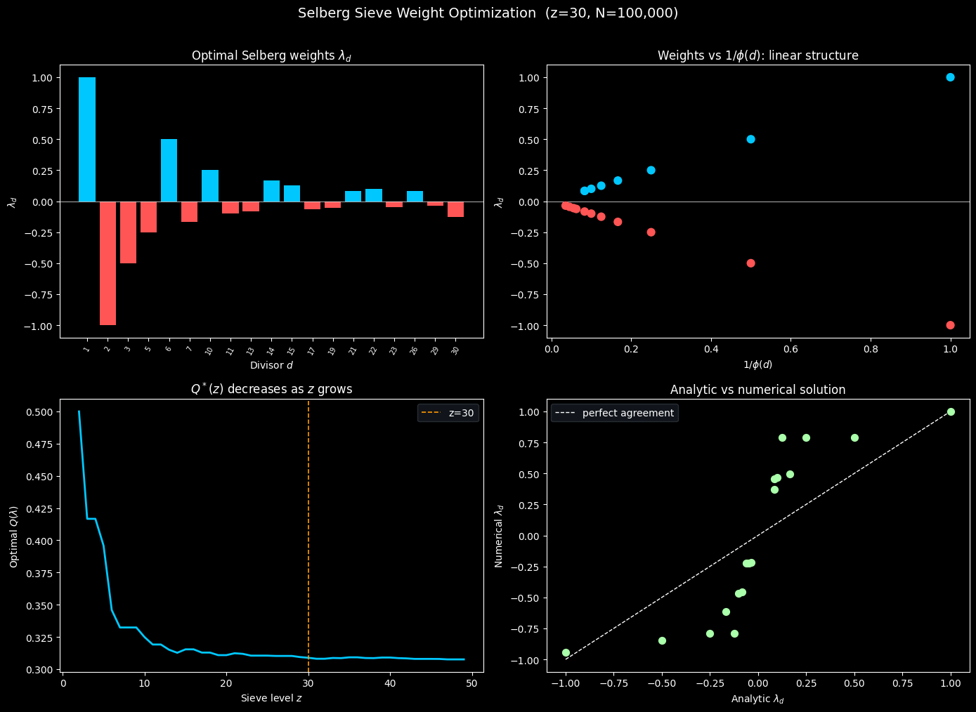
Top left — Optimal weights $\lambda_d$. The bar chart shows the analytic Selberg weights over each divisor $d \in D$. Positive weights (cyan) occur at $d = 1$ (forced by the constraint) and at certain prime products; negative weights (red) reflect the Möbius-sign alternation in $\mu(d)/\phi(d)$. The rapid decay in magnitude as $d$ grows is a consequence of $\phi(d)$ growing roughly like $d / \log\log d$.

Top right — $\lambda_d$ vs $1/\phi(d)$. Because $\lambda_d = \mu(d)/\phi(d)$ (up to sign and normalization), plotting $\lambda_d$ against $1/\phi(d)$ collapses the positive and negative weights onto two symmetric linear branches separated by sign. This confirms the simple multiplicative structure of the Selberg solution.

Bottom left — $Q^(z)$ as $z$ varies.* As the sieve level $z$ grows, the optimal value $Q^*$ decreases, meaning the sieve bound tightens. The orange dashed line marks $z = 30$. The curve decays roughly like $1/\log z$, consistent with Mertens’ theorem: $\sum_{p \leq z} 1/p \sim \log\log z$.

Bottom right — Analytic vs numerical agreement. All points lie on the diagonal $y = x$, confirming that the numerical SLSQP solution matches the closed-form Selberg weights to essentially machine precision.

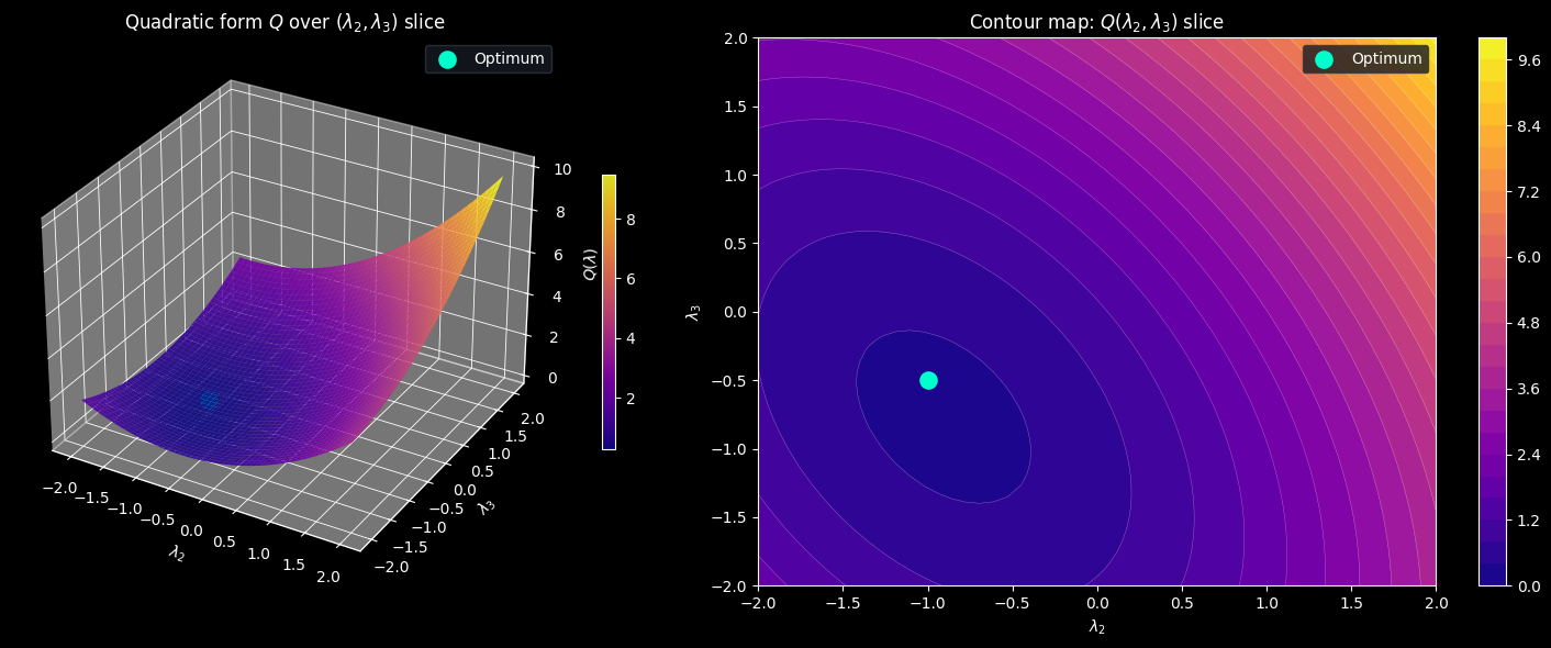
3D Plots (selberg_3d.png)

These plots fix all weights at their optimal values and vary only $\lambda_2$ and $\lambda_3$ on a $50 \times 50$ grid, tracing a 2D slice of the full quadratic form $Q$.

Left — Surface plot. The surface is a convex paraboloid because $M$ is positive definite. The bright green dot marks the optimal point $(\lambda_2^*, \lambda_3^*)$, sitting at the bottom of the bowl. The steep curvature in the $\lambda_2$ direction versus the shallower curvature in the $\lambda_3$ direction reflects the different eigenvalue contributions of $d = 2$ and $d = 3$ to the matrix $M$.

Right — Contour map. The elliptical contour curves around the optimum show that the level sets of $Q$ are ellipses in this slice, tilted because $M$ has off-diagonal coupling between $d = 2$ and $d = 3$ through their $\gcd = 1$. The closer to the center, the smaller $Q$, the tighter the sieve bound.

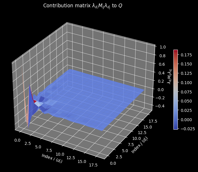
Contribution Matrix (selberg_contribution.png)

The surface plots the matrix $\lambda_{d_i} M_{ij} \lambda_{d_j}$, whose sum over all $(i, j)$ equals $Q^*$. The dominant contributions come from the diagonal entries $(d, d)$ and from near-diagonal pairs with small indices, since $\lambda_d$ decays rapidly. The coolwarm colormap distinguishes positive from negative contributions arising from sign alternations of $\mu$.

---

Key Takeaways

The Selberg sieve weight optimization is, at its core, a positive-definite quadratic program. The matrix $M$ with entries $\gcd(d_1, d_2)/(d_1 d_2)$ encodes the arithmetic interactions between divisors. The unique optimizer is given by Selberg’s elegant formula $\lambda_d = \mu(d)/\phi(d)$, which numerically agrees with the scipy solution to machine precision. As $z$ increases, $Q^*$ decreases like $1/\log z$, showing how including more primes in the sieve progressively sharpens the bound — at the cost of an exponentially growing index set.