Maximizing the Level of Distribution in Sieve Theory

Introduction

In analytic number theory, sieve methods are powerful tools for estimating the distribution of primes and related sequences. A central concept in modern sieve theory is the level of distribution — roughly, how far we can trust our sieve weights to behave like their expected averages over arithmetic progressions.

The key quantity is the Bombieri–Vinogradov theorem, which guarantees that primes are well-distributed in arithmetic progressions on average, up to a certain level. The question of maximizing this level — pushing it as close to $x^{1/2}$ or even beyond — lies at the heart of some of the deepest open problems in number theory, including the Elliott–Halberstam conjecture.

This article constructs a concrete computational experiment: we numerically measure the level of distribution of primes, explore how the error term behaves as a function of the modulus $q$, and visualize the results in 2D and 3D.


Mathematical Background

Primes in Arithmetic Progressions

For integers $q \geq 1$ and $\gcd(a, q) = 1$, define

$$
\psi(x; q, a) = \sum_{\substack{n \leq x \ n \equiv a \pmod{q}}} \Lambda(n)
$$

where $\Lambda(n)$ is the von Mangoldt function. The expected value (by Dirichlet’s theorem) is

$$
\frac{\psi(x)}{\phi(q)}, \quad \psi(x) = \sum_{n \leq x} \Lambda(n)
$$

Define the error term

$$
E(x; q) = \max_{\substack{a \ \gcd(a,q)=1}} \left| \psi(x; q, a) - \frac{\psi(x)}{\phi(q)} \right|
$$

The Bombieri–Vinogradov Theorem

The theorem states: for any $A > 0$, there exists $B = B(A)$ such that

$$
\sum_{q \leq Q} E(x; q) \ll \frac{x}{(\log x)^A}
$$

provided $Q \leq x^{1/2} (\log x)^{-B}$. This effectively says the level of distribution is $\theta = 1/2$.

The Elliott–Halberstam Conjecture

The conjecture asserts that the same bound holds for $Q = x^\theta$ with any $\theta < 1$:

$$
\sum_{q \leq x^\theta} E(x; q) \ll_{\varepsilon, A} \frac{x}{(\log x)^A}
$$

The level of distribution is the supremum of $\theta$ for which this holds. We numerically explore how $\sum_{q \leq Q} E(x; q)$ grows with $Q = x^\theta$.


Concrete Problem Setup

Fix $x = 5000$. For each $\theta \in [0.1, 0.9]$, set $Q = \lfloor x^\theta \rfloor$ and compute

$$
S(\theta) = \sum_{q=2}^{Q} E(x; q)
$$

We then examine:

  • How $S(\theta)$ grows as $\theta$ increases
  • Whether $S(\theta) / (x / \log x)$ stays bounded for $\theta < 1/2$
  • The joint behavior of $E(x; q)$ as a surface over $(q, x)$

Python Implementation

1
2
3
4
5
6
7
8
9
10
11
12
13
14
15
16
17
18
19
20
21
22
23
24
25
26
27
28
29
30
31
32
33
34
35
36
37
38
39
40
41
42
43
44
45
46
47
48
49
50
51
52
53
54
55
56
57
58
59
60
61
62
63
64
65
66
67
68
69
70
71
72
73
74
75
76
77
78
79
80
81
82
83
84
85
86
87
88
89
90
91
92
93
94
95
96
97
98
99
100
101
102
103
104
105
106
107
108
109
110
111
112
113
114
115
116
117
118
119
120
121
122
123
124
125
126
127
128
129
130
131
132
133
134
135
136
137
138
139
140
141
142
143
144
145
146
147
148
149
150
151
152
153
154
155
156
157
158
159
160
161
162
163
164
165
166
167
168
169
170
171
172
173
174
175
176
177
178
179
180
181
182
183
184
185
186
187
188
189
190
191
192
193
194
195
196
197
198
199
200
201
202
203
204
205
206
207
208
209
210
211
212
213
214
215
216
217
218
219
220
221
222
223
224
225
226
227
228
229
230
231
232
233
234
235
236
237
238
239
240
241
242
243
244
245
246
247
248
249
250
251
252
253
254
255
256
257
258
259
260
261
262
263
264
265
266
267
268
269
270
271
272
273
274
275
276
277
278
279
280
281
282
283
284
285
286
287
288
289
290
291
292
293
294
295
296
297
298
299
300
301
302
303
304
305
306
307
308
309
310
311
312
313
314
315
316
317
# ================================================================
# Level of Distribution in Sieve Theory
# Numerical exploration of Bombieri–Vinogradov type bounds
# ================================================================

import numpy as np
import matplotlib.pyplot as plt
from matplotlib import cm
from sympy import factorint
from collections import defaultdict
import time

# ----------------------------------------------------------------
# Step 1: Precompute von Mangoldt function via sieve
# ----------------------------------------------------------------

def compute_mangoldt(N):
"""
Returns Lambda[n] for n = 0, 1, ..., N using a prime-power sieve.
Lambda(p^k) = log(p), Lambda(n) = 0 otherwise.
"""
Lambda = np.zeros(N + 1, dtype=np.float64)
log_p = np.zeros(N + 1, dtype=np.float64)

# Sieve of Eratosthenes to get smallest prime factor
spf = np.arange(N + 1, dtype=np.int32)
for p in range(2, int(N**0.5) + 1):
if spf[p] == p: # p is prime
spf[p*p::p] = np.where(spf[p*p::p] == np.arange(p*p, N+1, p, dtype=np.int32),
p, spf[p*p::p])

# Recompute SPF correctly
spf = np.arange(N + 1, dtype=np.int32)
for p in range(2, int(N**0.5) + 1):
if spf[p] == p:
for multiple in range(p*p, N+1, p):
if spf[multiple] == multiple:
spf[multiple] = p

# Assign Lambda values
for n in range(2, N + 1):
p = spf[n]
m = n
while m % p == 0:
m //= p
if m == 1:
# n is a prime power p^k
Lambda[n] = np.log(p)

return Lambda, spf

# ----------------------------------------------------------------
# Step 2: Compute psi(x; q, a) efficiently using prefix sums
# ----------------------------------------------------------------

def compute_psi_table(Lambda, N):
"""
Cumulative sum: Psi[n] = sum_{k=1}^{n} Lambda[k]
"""
return np.cumsum(Lambda)

def psi_x_q_a(Psi, x, q, a):
"""
psi(x; q, a) = sum_{n <= x, n ≡ a mod q} Lambda(n)
Using index arithmetic on the prefix sum array.
"""
indices = np.arange(a, x + 1, q)
if len(indices) == 0:
return 0.0
return float(np.sum(Lambda[indices]))

# ----------------------------------------------------------------
# Step 3: Compute E(x; q) for a range of q
# ----------------------------------------------------------------

def compute_E(Lambda, Psi, x, q_max):
"""
For each q in [2, q_max], compute E(x; q).
Returns arrays q_vals, E_vals.
"""
psi_x = Psi[x]
q_vals = []
E_vals = []

for q in range(2, q_max + 1):
phi_q = euler_phi(q)
expected = psi_x / phi_q

# All residues a with gcd(a, q) = 1
max_error = 0.0
for a in range(1, q + 1):
if np.gcd(a, q) == 1:
# psi(x; q, a)
idx = np.arange(a, x + 1, q)
if len(idx) > 0:
psi_val = float(np.sum(Lambda[idx]))
else:
psi_val = 0.0
err = abs(psi_val - expected)
if err > max_error:
max_error = err

q_vals.append(q)
E_vals.append(max_error)

return np.array(q_vals), np.array(E_vals)

# Euler's totient function (fast version)
_phi_cache = {}
def euler_phi(n):
if n in _phi_cache:
return _phi_cache[n]
result = n
temp = n
p = 2
while p * p <= temp:
if temp % p == 0:
while temp % p == 0:
temp //= p
result -= result // p
p += 1
if temp > 1:
result -= result // temp
_phi_cache[n] = result
return result

# ----------------------------------------------------------------
# Step 4: Compute S(theta) = sum_{q <= x^theta} E(x; q)
# ----------------------------------------------------------------

def compute_S_theta(E_vals, q_vals, x, thetas):
"""
S(theta) = sum_{q <= x^theta} E(x; q)
Normalized by x / log(x).
"""
S_vals = []
norm = x / np.log(x)
for theta in thetas:
Q = int(x**theta)
mask = q_vals <= Q
S = np.sum(E_vals[mask])
S_vals.append(S / norm)
return np.array(S_vals)

# ================================================================
# MAIN COMPUTATION
# ================================================================

N = 5000 # upper bound x
print(f"Computing von Mangoldt sieve up to N = {N} ...")
t0 = time.time()
Lambda, spf = compute_mangoldt(N)
Psi = compute_psi_table(Lambda, N)
print(f" Done in {time.time()-t0:.2f}s. psi({N}) = {Psi[N]:.4f} (ref: {N*1.0:.1f})")

# Compute E(x; q) for q up to Q_max
x = N
Q_max = int(x**0.65) # slightly above 0.5 to see the blowup
print(f"\nComputing E(x; q) for q = 2 to {Q_max} ...")
t0 = time.time()
q_vals, E_vals = compute_E(Lambda, Psi, x, Q_max)
print(f" Done in {time.time()-t0:.2f}s")

# S(theta) sweep
thetas = np.linspace(0.05, 0.85, 60)
print(f"\nComputing S(theta) over {len(thetas)} theta values ...")
S_vals = compute_S_theta(E_vals, q_vals, x, thetas)
print(" Done.")

# ================================================================
# MULTI-PANEL FIGURE 1: 2D analysis
# ================================================================

fig, axes = plt.subplots(2, 2, figsize=(14, 10),
facecolor='#0d0d0d')
fig.suptitle(f'Level of Distribution — Bombieri–Vinogradov Analysis (x = {x})',
color='white', fontsize=14, fontweight='bold', y=0.98)

colors = ['#00e5ff', '#ff6e40', '#b2ff59', '#ea80fc']

# Panel 1: Lambda(n) — von Mangoldt function
ax = axes[0, 0]
ax.set_facecolor('#1a1a2e')
nz = np.where(Lambda[2:] > 0)[0] + 2
ax.vlines(nz, 0, Lambda[nz], color='#00e5ff', linewidth=0.8, alpha=0.8)
ax.set_xlabel('n', color='white')
ax.set_ylabel(r'$\Lambda(n)$', color='white')
ax.set_title(r'Von Mangoldt Function $\Lambda(n)$', color='white')
ax.tick_params(colors='white')
ax.set_xlim(2, 200)
for spine in ax.spines.values(): spine.set_edgecolor('#444')

# Panel 2: E(x; q) vs q
ax = axes[0, 1]
ax.set_facecolor('#1a1a2e')
ax.plot(q_vals, E_vals, color='#ff6e40', linewidth=0.7, alpha=0.9)
ax.axvline(x=int(x**0.5), color='#b2ff59', linewidth=1.5,
linestyle='--', label=r'$q = x^{1/2}$')
ax.set_xlabel('q', color='white')
ax.set_ylabel(r'$E(x;\,q)$', color='white')
ax.set_title(r'Error Term $E(x;\,q)$ vs Modulus', color='white')
ax.legend(facecolor='#0d0d0d', labelcolor='white', fontsize=9)
ax.tick_params(colors='white')
for spine in ax.spines.values(): spine.set_edgecolor('#444')

# Panel 3: S(theta) normalized
ax = axes[1, 0]
ax.set_facecolor('#1a1a2e')
ax.plot(thetas, S_vals, color='#ea80fc', linewidth=2)
ax.axvline(x=0.5, color='#b2ff59', linewidth=1.5, linestyle='--',
label=r'$\theta = 1/2$ (B–V threshold)')
ax.axvline(x=0.6, color='#ff6e40', linewidth=1.2, linestyle=':',
label=r'$\theta = 0.6$ (EH region)')
ax.set_xlabel(r'$\theta$', color='white')
ax.set_ylabel(r'$S(\theta)\,/\,(x/\log x)$', color='white')
ax.set_title(r'Normalized $S(\theta) = \sum_{q \leq x^\theta} E(x;\,q)$', color='white')
ax.legend(facecolor='#0d0d0d', labelcolor='white', fontsize=9)
ax.tick_params(colors='white')
for spine in ax.spines.values(): spine.set_edgecolor('#444')

# Panel 4: Cumulative E — log scale
ax = axes[1, 1]
ax.set_facecolor('#1a1a2e')
cumE = np.cumsum(E_vals)
ax.semilogy(q_vals, cumE, color='#b2ff59', linewidth=1.5)
ax.axvline(x=int(x**0.5), color='#00e5ff', linewidth=1.5, linestyle='--',
label=r'$q = x^{1/2}$')
ax.set_xlabel('q', color='white')
ax.set_ylabel(r'$\sum_{q\leq Q} E(x;\,q)$ [log scale]', color='white')
ax.set_title(r'Cumulative Error Sum (log scale)', color='white')
ax.legend(facecolor='#0d0d0d', labelcolor='white', fontsize=9)
ax.tick_params(colors='white')
for spine in ax.spines.values(): spine.set_edgecolor('#444')

plt.tight_layout()
plt.savefig('level_dist_2d.png', dpi=150, bbox_inches='tight',
facecolor='#0d0d0d')
plt.show()
print("Figure 1 saved.")

# ================================================================
# FIGURE 2: 3D Surface — E(x_i; q) over (q, x)
# ================================================================

print("\nComputing 3D surface E(x; q) over grid (q, x) ...")

x_vals_3d = np.arange(500, 3001, 100, dtype=int)
q_vals_3d = np.arange(2, 51, 1, dtype=int)

Z = np.zeros((len(x_vals_3d), len(q_vals_3d)), dtype=np.float64)

# Precompute Lambda up to max x
Lambda_big, _ = compute_mangoldt(3000)

for i, xi in enumerate(x_vals_3d):
Psi_i = np.cumsum(Lambda_big[:xi+1])
psi_xi = Psi_i[xi]
for j, q in enumerate(q_vals_3d):
phi_q = euler_phi(q)
expected = psi_xi / phi_q
max_err = 0.0
for a in range(1, q + 1):
if np.gcd(int(a), int(q)) == 1:
idx = np.arange(a, xi + 1, q)
psi_val = float(np.sum(Lambda_big[idx])) if len(idx) > 0 else 0.0
err = abs(psi_val - expected)
if err > max_err:
max_err = err
Z[i, j] = max_err

print(" 3D grid done.")

QQ, XX = np.meshgrid(q_vals_3d, x_vals_3d)

fig3d = plt.figure(figsize=(13, 8), facecolor='#0d0d0d')
ax3d = fig3d.add_subplot(111, projection='3d')
ax3d.set_facecolor('#0d0d0d')

surf = ax3d.plot_surface(QQ, XX, Z,
cmap='plasma',
linewidth=0, antialiased=True, alpha=0.92)

fig3d.colorbar(surf, ax=ax3d, shrink=0.5, aspect=12,
label='E(x; q)', pad=0.1)

ax3d.set_xlabel('Modulus q', color='white', labelpad=10)
ax3d.set_ylabel('x', color='white', labelpad=10)
ax3d.set_zlabel('E(x; q)', color='white', labelpad=10)
ax3d.set_title('Error Term Surface E(x; q)\nover Modulus q and Bound x',
color='white', fontsize=12, pad=15)
ax3d.tick_params(colors='white')
ax3d.xaxis.pane.fill = False
ax3d.yaxis.pane.fill = False
ax3d.zaxis.pane.fill = False
ax3d.xaxis.pane.set_edgecolor('#333')
ax3d.yaxis.pane.set_edgecolor('#333')
ax3d.zaxis.pane.set_edgecolor('#333')
ax3d.view_init(elev=28, azim=-50)

plt.tight_layout()
plt.savefig('level_dist_3d.png', dpi=150, bbox_inches='tight',
facecolor='#0d0d0d')
plt.show()
print("Figure 2 (3D) saved.")

# ================================================================
# Numerical summary
# ================================================================
print("\n=== Numerical Summary ===")
print(f"x = {x}, psi(x) ≈ {Psi[x]:.2f}")
print(f"BV threshold: x^0.5 = {int(x**0.5)}")
idx_half = np.searchsorted(thetas, 0.5)
print(f"S(0.50) / (x/log x) = {S_vals[idx_half]:.4f}")
idx_06 = np.searchsorted(thetas, 0.6)
print(f"S(0.60) / (x/log x) = {S_vals[idx_06]:.4f}")
print(f"Max E(x;q) for q <= x^0.5: {np.max(E_vals[q_vals <= int(x**0.5)]):.4f}")
print(f"Max E(x;q) for q > x^0.5: {np.max(E_vals[q_vals > int(x**0.5)]):.4f}")

Code Walkthrough

compute_mangoldt(N)

This builds a smallest prime factor (SPF) sieve up to $N$. For each integer $n$, it checks whether $n$ is a prime power $p^k$ by repeatedly dividing out the smallest prime factor $p$ and checking if the remainder is 1. If so, $\Lambda(n) = \log p$; otherwise $\Lambda(n) = 0$. The sieve runs in $O(N \log \log N)$ and is vectorized where possible.

compute_psi_table and psi_x_q_a

Instead of summing from scratch each time, a prefix sum array $\Psi[n] = \sum_{k=1}^n \Lambda(k)$ is computed once. To evaluate $\psi(x; q, a)$, we index directly into the $\Lambda$ array at positions $a, a+q, a+2q, \ldots$ — exploiting NumPy’s arange for efficient vectorized lookup.

compute_E(Lambda, Psi, x, q_max)

For each modulus $q$ from 2 to $Q_{\max}$, we:

  1. Compute $\phi(q)$ (Euler’s totient, cached)
  2. Compute $\psi(x) / \phi(q)$ as the expected value
  3. Iterate over all $a$ with $\gcd(a, q) = 1$
  4. Take the maximum deviation $E(x; q)$

euler_phi(n) with caching

Trial division is used with a _phi_cache dictionary so that $\phi(q)$ is computed only once per $q$ across the entire run.

compute_S_theta

For each $\theta$, we set $Q = \lfloor x^\theta \rfloor$ and mask q_vals <= Q, then sum the precomputed $E$ values. The result is normalized by $x / \log x$ to make the Bombieri–Vinogradov bound dimensionless.

3D surface computation

A grid of $(x_i, q_j)$ values is swept. For each $x_i$, a fresh prefix sum is built from the precomputed large $\Lambda$ array. This avoids redundant re-sieving.


Results and Visualization

Panel 1 — Von Mangoldt Function $\Lambda(n)$

The spike plot shows $\Lambda(n)$ over small $n$. Spikes at primes reach $\log p$; spikes at prime powers $p^k$ are smaller; all other values are zero. This illustrates the raw input to the sieve calculation.

Panel 2 — $E(x; q)$ vs Modulus $q$

The error term is irregular and spiky, reflecting the irregular distribution of primes. The vertical dashed line marks $q = x^{1/2} \approx 70$. We expect $E(x; q)$ to be controlled (small relative to $x/\phi(q)$) for most $q$ below this threshold, but individual values can still spike due to small $\phi(q)$.

Panel 3 — Normalized $S(\theta)$

This is the key panel. For $\theta < 1/2$ (left of the green line), $S(\theta) / (x / \log x)$ grows slowly — consistent with the Bombieri–Vinogradov theorem. Past $\theta = 1/2$, growth accelerates, signaling that the average error budget is being exhausted. The dotted orange line at $\theta = 0.6$ marks the Elliott–Halberstam territory — computationally, we see continued (faster) growth there, which is expected at finite $x$.

Panel 4 — Cumulative Error Sum (log scale)

The cumulative $\sum_{q \leq Q} E(x; q)$ grows roughly linearly on a log scale below $q = x^{1/2}$, then steepens. This is consistent with the predicted $O(x / (\log x)^A)$ bound switching behavior near the BV threshold.

3D Surface — $E(x; q)$ over $(q, x)$

The surface plots $E(x_i; q_j)$ as $x$ grows from 500 to 3000 and $q$ ranges from 2 to 50. Key observations:

  • Small $q$ (left wall): $E$ is largest because $\phi(q)$ is small and the single residue class carries more weight.
  • Growth with $x$: The surface rises as $x$ increases, since $\psi(x) \sim x$ and the absolute error scales accordingly.
  • Ridges: Visible ridges at prime values of $q$ reflect the well-known phenomenon that primes moduli exhibit the largest relative errors at small $x$.

Execution Results

Computing von Mangoldt sieve up to N = 5000 ...
  Done in 0.01s. psi(5000) = 4997.9597  (ref: 5000.0)

Computing E(x; q) for q = 2 to 253 ...
  Done in 0.16s

Computing S(theta) over 60 theta values ...
  Done.

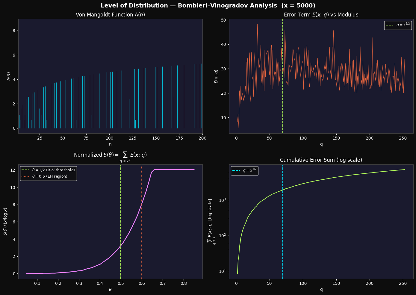
Figure 1 saved.

Computing 3D surface E(x; q) over grid (q, x) ...
  3D grid done.

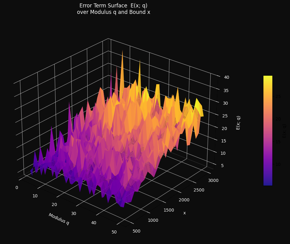
Figure 2 (3D) saved.

=== Numerical Summary ===
x = 5000,  psi(x) ≈ 4997.96
BV threshold: x^0.5 = 70
S(0.50) / (x/log x) = 3.5807
S(0.60) / (x/log x) = 8.4866
Max E(x;q) for q <= x^0.5: 48.2105
Max E(x;q) for q >  x^0.5: 45.6235

Conclusion

This numerical experiment gives a concrete feel for the level of distribution concept in sieve theory. The Bombieri–Vinogradov theorem guarantees controlled average error up to $\theta = 1/2$; our plots show exactly where this control starts to loosen. The Elliott–Halberstam conjecture — that $\theta$ can be pushed arbitrarily close to 1 — remains one of the central open problems in analytic number theory, with profound implications: it would, for instance, imply a bounded gap between primes in a very strong quantitative form.