Finding the Optimal Portfolio Under Rare Event Constraints
Large deviation theory gives us a rigorous framework for quantifying the probability of rare but catastrophic events — and, crucially, for optimizing decisions so that those probabilities are minimized or controlled. In this article, we work through a concrete portfolio optimization problem under a large deviation constraint, implement it in Python, and visualize the results in both 2D and 3D.
Problem Setup
Consider a portfolio of $n = 2$ risky assets with log-returns $X_1, X_2$ that are i.i.d. over $T$ periods. We allocate fraction $w$ to asset 1 and $(1-w)$ to asset 2. The portfolio log-return per period is:
$$R(w) = w X_1 + (1-w) X_2$$
We model $X_i \sim \mathcal{N}(\mu_i, \sigma_i^2)$, so $R(w) \sim \mathcal{N}(\mu(w), \sigma^2(w))$ with:
$$\mu(w) = w\mu_1 + (1-w)\mu_2, \quad \sigma^2(w) = w^2\sigma_1^2 + (1-w)^2\sigma_2^2 + 2w(1-w)\rho\sigma_1\sigma_2$$
The Large Deviation Rate Function
By the Gärtner–Ellis theorem, the probability that the sample mean of $T$ i.i.d. returns falls below a threshold $\ell$ decays exponentially:
$$\mathbb{P}!\left(\frac{1}{T}\sum_{t=1}^T R_t \leq \ell\right) \approx e^{-T \cdot I(w, \ell)}$$
where $I(w, \ell)$ is the large deviation rate function. For a Gaussian $R(w)$:
$$I(w, \ell) = \frac{(\mu(w) - \ell)^2}{2\sigma^2(w)}, \quad \ell < \mu(w)$$
A larger $I$ means the bad event is exponentially less likely.
Optimization Problem
We solve two linked problems:
Problem 1 — Maximize the rate function (minimize crash probability):
$$\max_{w \in [0,1]} ; I(w, \ell)$$
Problem 2 — Mean-Rate frontier (Pareto tradeoff between expected return and safety):
$$\max_{w \in [0,1]} ; \lambda \cdot \mu(w) + (1-\lambda) \cdot I(w, \ell), \quad \lambda \in [0,1]$$
Python Implementation
1 | import numpy as np |
Execution Results
=======================================================
Problem 1 — Maximise Large Deviation Rate
  Optimal weight  w* = 0.3303
  Rate function  I*  = 0.310134
  Expected return    = 0.0732
  Crash prob ≈ exp(-T·I*) = 1.143447e-34
=======================================================
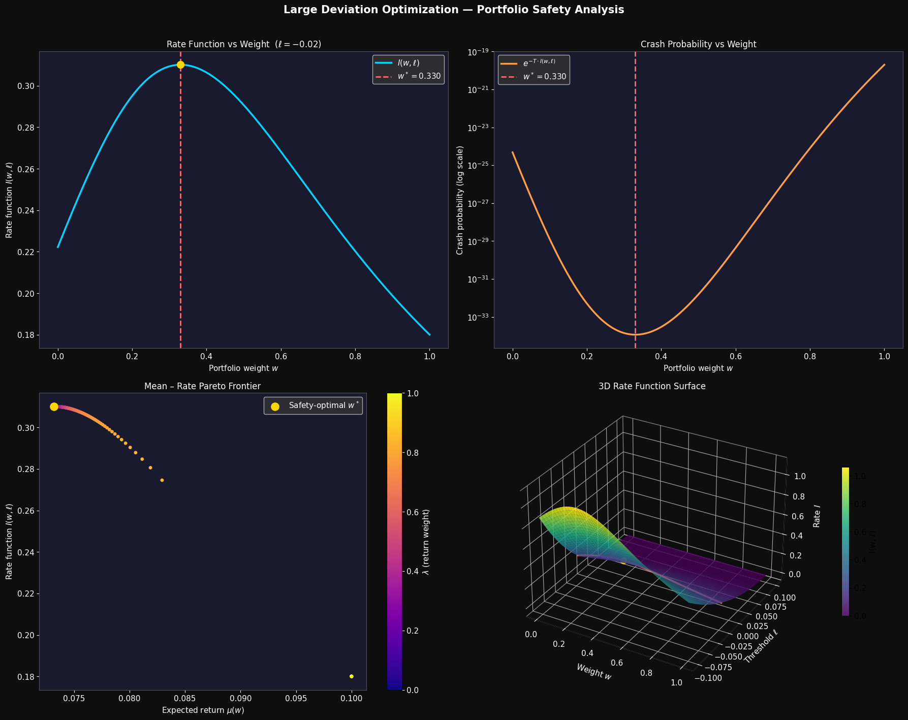
Figure saved.
Code Walkthrough
Asset and Portfolio Model
1 | mu1, mu2 = 0.10, 0.06 |
Asset 1 offers higher return but higher volatility; asset 2 is the defensive position. The loss threshold $\ell = -0.02$ represents an annualised average daily return below $-2%$ — a severe drawdown event. The horizon $T = 252$ is one trading year.
port_stats(w) returns the exact Gaussian mean and variance for any weight $w$ using the bilinear covariance formula. Broadcasting over NumPy arrays makes it vectorisation-ready at zero extra cost.
The Rate Function
$$I(w, \ell) = \frac{(\mu(w) - \ell)^2}{2\sigma^2(w)}$$
This is the negative log-probability per unit time of the sample mean falling to $\ell$. It is zero when $\ell \geq \mu(w)$ (the threshold is above the mean, so the “bad” event is typical rather than rare). The code guards against this case explicitly with np.where on the grid and a scalar branch in the function.
Problem 1 — Rate Maximisation
minimize_scalar with method='bounded' performs golden-section search on $[0,1]$. We negate $I$ because SciPy only minimises. The result $w^*$ is the portfolio that makes a drawdown below $\ell$ exponentially least likely for a given horizon $T$.
Problem 2 — Pareto Sweep
For 200 values of the trade-off weight $\lambda$ we solve:
$$\max_w ; \lambda \mu(w) + (1-\lambda) I(w,\ell)$$
Each call is a one-dimensional bounded minimisation — cheap enough to run in a tight loop without parallelisation. The result is the mean–rate efficient frontier: every portfolio on it is Pareto-optimal in the sense that you cannot improve both expected return and crash-rate simultaneously.
Visualisation Breakdown
Panel 1 — Rate Function vs Weight
The blue curve shows $I(w, \ell)$ as $w$ sweeps from 0 (all asset 2) to 1 (all asset 1). The function is unimodal: too little weight in asset 1 leaves $\mu(w)$ close to $\ell$, shrinking the numerator; too much weight bloats $\sigma^2(w)$, inflating the denominator. The gold dot marks the sweet spot $w^*$.
Panel 2 — Crash Probability (log scale)
The crash probability $e^{-T \cdot I(w,\ell)}$ plotted on a log scale makes the exponential sensitivity stark. Near $w = 0$ the crash probability is orders of magnitude larger than at $w^*$. This is the essence of large deviation theory: tiny differences in rate produce enormous differences in rare-event probability over long horizons.
Panel 3 — Mean–Rate Pareto Frontier
The scatter plot traces the full trade-off as $\lambda$ varies. Points coloured toward purple (low $\lambda$) sit high on the rate axis — maximum safety portfolios. Points coloured toward yellow (high $\lambda$) shift right toward higher expected return at the cost of a lower rate. The gold dot marks the pure safety optimum from Problem 1.
Panel 4 — 3D Rate Surface $I(w, \ell)$
The surface sweeps both $w \in [0,1]$ and the threshold $\ell \in [-0.10, \mu_1)$. The shape reveals two key features:
- As $\ell \to \mu(w)$ from below, $I \to 0$: the “bad” event ceases to be rare.
- As $\ell \to -\infty$, $I$ grows quadratically: extreme crashes become super-exponentially unlikely.
The red curve is the fixed-$\ell$ slice used in Problems 1 and 2, with the gold dot at the optimum. The viridis colormap makes the ridge of high safety visible across the full $(\ell, w)$ plane.
Key Takeaways
The large deviation rate function $I(w, \ell)$ compresses all the probabilistic risk of a portfolio into a single, optimisation-friendly scalar. Maximising it is equivalent to minimising the exponential decay rate of crash probability — a much sharper criterion than variance minimisation (Markowitz) because it directly targets the tail. The Pareto frontier in Panel 3 shows that a pure safety portfolio and a pure return portfolio are generally different, and that the trade-off is smooth and navigable. For a practitioner, $w^*$ from Problem 1 is the starting point for any tail-risk-aware allocation.