Minimizing the Error Term of the Chebyshev Function ψ(x)

Introduction

The Chebyshev ψ (psi) function is one of the most important objects in analytic number theory. Defined as

$$\psi(x) = \sum_{p^k \leq x} \log p$$

where the sum runs over all prime powers $p^k$ not exceeding $x$, it encodes deep information about the distribution of primes. The Prime Number Theorem (PNT) is equivalent to the statement that

$$\psi(x) \sim x \quad \text{as } x \to \infty$$

But how fast does $\psi(x)$ approach $x$? The error term

$$E(x) = \psi(x) - x$$

is the heart of the matter, and its behavior is intimately connected to the Riemann Hypothesis (RH). Under RH, one expects

$$E(x) = O!\left(\sqrt{x} \log^2 x\right)$$

In this article, we pose a concrete optimization problem: given a finite truncation of the explicit formula

$$\psi(x) = x - \sum_{\rho} \frac{x^\rho}{\rho} - \log(2\pi) - \frac{1}{2}\log!\left(1 - x^{-2}\right)$$

where $\rho = \frac{1}{2} + i\gamma$ are non-trivial zeros of the Riemann zeta function, we minimize the integrated squared error

$$\mathcal{L}(\mathbf{w}) = \int_{2}^{X} \left( \psi(x) - x + \sum_{k=1}^{N} w_k \cdot \frac{2\sqrt{x}\cos(\gamma_k \log x)}{\gamma_k} \right)^2 dx$$

by learning optimal weights $\mathbf{w} = (w_1, \dots, w_N)$ for the zero contributions.


Mathematical Background

The Explicit Formula

Riemann’s explicit formula connects $\psi(x)$ to the zeros of $\zeta(s)$. For $x > 1$ not a prime power:

$$\psi(x) = x - \sum_{\rho} \frac{x^\rho}{\rho} - \log(2\pi) - \frac{1}{2}\log!\left(1-x^{-2}\right)$$

Pairing conjugate zeros $\rho = \frac{1}{2} + i\gamma$ and $\bar{\rho} = \frac{1}{2} - i\gamma$:

$$\frac{x^\rho}{\rho} + \frac{x^{\bar\rho}}{\bar\rho} = \frac{2\sqrt{x}\left[\cos(\gamma\log x) \cdot \frac{1}{2} + \gamma\sin(\gamma\log x)\right]}{\frac{1}{4}+\gamma^2}$$

which we abbreviate as a zero contribution $Z_k(x)$.

The Optimization Problem

We parameterize the truncated approximation:

$$\hat\psi(x; \mathbf{w}) = x - \sum_{k=1}^{N} w_k Z_k(x)$$

and minimize the mean squared error over $x \in [2, X]$:

$$\mathcal{L}(\mathbf{w}) = \frac{1}{X-2}\int_{2}^{X} \left(\psi(x) - \hat\psi(x;\mathbf{w})\right)^2 dx$$

The baseline (all $w_k = 1$) corresponds to the classical explicit formula. We solve for the optimal $\mathbf{w}^*$ via least squares on a discrete grid, then compare errors.


Python Implementation

1
2
3
4
5
6
7
8
9
10
11
12
13
14
15
16
17
18
19
20
21
22
23
24
25
26
27
28
29
30
31
32
33
34
35
36
37
38
39
40
41
42
43
44
45
46
47
48
49
50
51
52
53
54
55
56
57
58
59
60
61
62
63
64
65
66
67
68
69
70
71
72
73
74
75
76
77
78
79
80
81
82
83
84
85
86
87
88
89
90
91
92
93
94
95
96
97
98
99
100
101
102
103
104
105
106
107
108
109
110
111
112
113
114
115
116
117
118
119
120
121
122
123
124
125
126
127
128
129
130
131
132
133
134
135
136
137
138
139
140
141
142
143
144
145
146
147
148
149
150
151
152
153
154
155
156
157
158
159
160
161
162
163
164
165
166
167
168
169
170
171
172
173
174
175
176
177
178
179
180
181
182
183
184
185
186
187
188
189
190
191
192
193
194
195
196
197
198
199
200
201
202
203
204
205
206
207
208
209
210
211
212
213
214
215
216
217
218
219
220
221
222
223
224
225
226
227
228
229
# ============================================================
# Chebyshev psi function: error term minimization
# via explicit formula zero weighting
# ============================================================

import numpy as np
import matplotlib.pyplot as plt
from matplotlib import cm
from scipy.optimize import least_squares
from mpl_toolkits.mplot3d import Axes3D
import warnings
warnings.filterwarnings("ignore")

# ── Dark theme ──────────────────────────────────────────────
plt.rcParams.update({
"figure.facecolor": "#0d1117",
"axes.facecolor": "#161b22",
"axes.edgecolor": "#30363d",
"axes.labelcolor": "#c9d1d9",
"xtick.color": "#c9d1d9",
"ytick.color": "#c9d1d9",
"text.color": "#c9d1d9",
"grid.color": "#21262d",
"grid.linestyle": "--",
"legend.facecolor": "#161b22",
"legend.edgecolor": "#30363d",
})

# ── 1. Riemann zeta non-trivial zeros (imaginary parts γ_k) ─
# First 30 zeros from published tables
ZEROS = np.array([
14.134725, 21.022040, 25.010858, 30.424876, 32.935062,
37.586178, 40.918719, 43.327073, 48.005151, 49.773832,
52.970321, 56.446248, 59.347044, 60.831779, 65.112544,
67.079811, 69.546402, 72.067158, 75.704691, 77.144840,
79.337375, 82.910381, 84.735493, 87.425275, 88.809112,
92.491899, 94.651344, 95.870634, 98.831194, 101.317851,
])

# ── 2. True Chebyshev ψ(x) via sieve ───────────────────────
def sieve_primes(n):
"""Return sorted array of primes up to n."""
sieve = np.ones(n + 1, dtype=bool)
sieve[0:2] = False
for i in range(2, int(n**0.5) + 1):
if sieve[i]:
sieve[i*i::i] = False
return np.where(sieve)[0]

def chebyshev_psi(x_vals, primes):
"""
Compute ψ(x) for each x in x_vals.
ψ(x) = Σ_{p^k ≤ x} log(p)
Vectorized over x_vals.
"""
psi = np.zeros(len(x_vals))
log_primes = np.log(primes)
for i, x in enumerate(x_vals):
# sum log p for all prime powers p^k <= x
total = 0.0
for p, lp in zip(primes, log_primes):
if p > x:
break
pk = p
while pk <= x:
total += lp
pk *= p
psi[i] = total
return psi

# ── 3. Zero contribution Z_k(x) ────────────────────────────
def zero_contribution(x, gamma):
"""
Paired contribution from zeros ρ = 1/2 ± iγ:
Z(x; γ) = 2√x [cos(γ log x)/2 + γ sin(γ log x)] / (1/4 + γ²)
= 2√x [0.5·cos(γ log x) + γ·sin(γ log x)] / (0.25 + γ²)
"""
log_x = np.log(x)
sqrt_x = np.sqrt(x)
denom = 0.25 + gamma**2
return 2 * sqrt_x * (0.5 * np.cos(gamma * log_x) + gamma * np.sin(gamma * log_x)) / denom

# ── 4. Grid setup ───────────────────────────────────────────
X_MAX = 200 # upper limit of integration
N_GRID = 800 # number of x evaluation points
N_ZEROS = 20 # number of zero pairs to use

x_grid = np.linspace(2.5, X_MAX, N_GRID)
primes = sieve_primes(int(X_MAX) + 10)
gammas = ZEROS[:N_ZEROS]

print(f"Computing ψ(x) on {N_GRID} points up to x = {X_MAX} ...")
psi_true = chebyshev_psi(x_grid, primes)
print("Done.")

# ── 5. Build design matrix A ───────────────────────────────
# Each column: Z_k(x_grid)
# residual = psi_true - x_grid + A @ w → minimize ||psi_true - x_grid + A @ w||
# Equivalently: A @ w ≈ -(psi_true - x_grid) = x_grid - psi_true

A = np.column_stack([zero_contribution(x_grid, g) for g in gammas])

# ── 6. Baseline: w = 1 (classical explicit formula) ─────────
baseline_residual = psi_true - (x_grid - A @ np.ones(N_ZEROS))
baseline_mse = np.mean(baseline_residual**2)
print(f"Baseline MSE (w=1): {baseline_mse:.4f}")

# ── 7. Least-squares optimization ───────────────────────────
# Solve: A @ w ≈ x_grid - psi_true (in least-squares sense)
target = x_grid - psi_true
result = np.linalg.lstsq(A, target, rcond=None)
w_opt = result[0]

opt_residual = psi_true - (x_grid - A @ w_opt)
opt_mse = np.mean(opt_residual**2)
print(f"Optimized MSE (w=w*): {opt_mse:.4f}")
print(f"MSE reduction: {100*(1 - opt_mse/baseline_mse):.2f}%")

# ── 8. Reconstruction ───────────────────────────────────────
psi_baseline = x_grid - A @ np.ones(N_ZEROS)
psi_opt = x_grid - A @ w_opt

# ── 9. Plot 1 – ψ(x) vs approximations ─────────────────────
fig, axes = plt.subplots(2, 1, figsize=(13, 9))
fig.suptitle(r"Chebyshev $\psi(x)$: Explicit Formula & Error Minimization",
fontsize=15, fontweight="bold", color="#f0f6fc")

ax = axes[0]
ax.plot(x_grid, psi_true, color="#58a6ff", lw=1.8, label=r"True $\psi(x)$", zorder=3)
ax.plot(x_grid, x_grid, color="#3fb950", lw=1.2, ls="--", label=r"$x$ (PNT)", zorder=2)
ax.plot(x_grid, psi_baseline, color="#f78166", lw=1.2, ls="-.", label=r"Explicit ($w=1$)", zorder=2)
ax.plot(x_grid, psi_opt, color="#ffa657", lw=1.6, label=r"Optimized ($w^*$)", zorder=4)
ax.set_xlabel(r"$x$", fontsize=12)
ax.set_ylabel(r"$\psi(x)$", fontsize=12)
ax.legend(fontsize=10)
ax.grid(True)
ax.set_title(r"$\psi(x)$ and its approximations", fontsize=12)

ax = axes[1]
ax.plot(x_grid, baseline_residual, color="#f78166", lw=1.2, label=r"$E(x)$ baseline ($w=1$)")
ax.plot(x_grid, opt_residual, color="#ffa657", lw=1.6, label=r"$E(x)$ optimized ($w^*$)")
ax.axhline(0, color="#8b949e", lw=0.8)
ax.fill_between(x_grid, opt_residual, alpha=0.15, color="#ffa657")
ax.set_xlabel(r"$x$", fontsize=12)
ax.set_ylabel(r"$E(x) = \psi(x) - \hat\psi(x)$", fontsize=12)
ax.legend(fontsize=10)
ax.grid(True)
ax.set_title("Error term comparison", fontsize=12)

plt.tight_layout()
plt.savefig("psi_error_comparison.png", dpi=150, bbox_inches="tight",
facecolor=fig.get_facecolor())
plt.show()
print("[Figure 1 saved]")

# ── 10. Plot 2 – Optimal weights w* ─────────────────────────
fig, ax = plt.subplots(figsize=(13, 5))
fig.patch.set_facecolor("#0d1117")
ax.set_facecolor("#161b22")

colors_w = np.where(w_opt >= 1, "#3fb950", "#f78166")
bars = ax.bar(np.arange(N_ZEROS), w_opt, color=colors_w, edgecolor="#21262d", linewidth=0.5)
ax.axhline(1.0, color="#58a6ff", lw=1.5, ls="--", label=r"Baseline $w_k=1$")
ax.set_xlabel(r"Zero index $k$", fontsize=12)
ax.set_ylabel(r"Optimal weight $w_k^*$", fontsize=12)
ax.set_xticks(np.arange(N_ZEROS))
ax.set_xticklabels([f"{g:.2f}" for g in gammas], rotation=60, fontsize=7)
ax.legend(fontsize=10)
ax.grid(True, axis="y")
ax.set_title(r"Optimal weights $w^*$ per Riemann zero $\gamma_k$", fontsize=13,
fontweight="bold", color="#f0f6fc")

plt.tight_layout()
plt.savefig("psi_optimal_weights.png", dpi=150, bbox_inches="tight",
facecolor=fig.get_facecolor())
plt.show()
print("[Figure 2 saved]")

# ── 11. Plot 3 – 3D: Error surface vs N_zeros & x ───────────
# Sweep number of zeros N = 1..20 and see how MSE changes with x
N_sweep = np.arange(1, N_ZEROS + 1)
x_coarse = x_grid[::8] # thin grid for 3D
E_surface = np.zeros((len(N_sweep), len(x_coarse)))

for ni, n in enumerate(N_sweep):
An = A[:, :n]
tgt_n = x_grid - psi_true
wn = np.linalg.lstsq(An, tgt_n, rcond=None)[0]
res_n = psi_true - (x_grid - An @ wn)
E_surface[ni, :] = res_n[::8]

X3d, Y3d = np.meshgrid(x_coarse, N_sweep)
Z3d = np.abs(E_surface)

fig3 = plt.figure(figsize=(14, 8))
fig3.patch.set_facecolor("#0d1117")
ax3 = fig3.add_subplot(111, projection="3d")
ax3.set_facecolor("#161b22")

surf = ax3.plot_surface(X3d, Y3d, Z3d,
cmap="plasma", alpha=0.88,
linewidth=0, antialiased=True)
ax3.set_xlabel(r"$x$", fontsize=11, color="#c9d1d9", labelpad=8)
ax3.set_ylabel(r"Num zeros $N$", fontsize=11, color="#c9d1d9", labelpad=8)
ax3.set_zlabel(r"$|E(x)|$", fontsize=11, color="#c9d1d9", labelpad=8)
ax3.set_title(r"3D Error Surface $|E(x)|$ vs $x$ and number of zeros used",
fontsize=12, fontweight="bold", color="#f0f6fc", pad=15)
ax3.tick_params(colors="#c9d1d9")
fig3.colorbar(surf, ax=ax3, pad=0.1, shrink=0.55, label=r"$|E(x)|$")

plt.tight_layout()
plt.savefig("psi_3d_error_surface.png", dpi=150, bbox_inches="tight",
facecolor=fig3.get_facecolor())
plt.show()
print("[Figure 3 saved]")

# ── 12. Summary statistics ───────────────────────────────────
print("\n" + "="*55)
print(" SUMMARY")
print("="*55)
print(f" x range : [2.5, {X_MAX}]")
print(f" Grid points : {N_GRID}")
print(f" Zeros used : {N_ZEROS}")
print(f" Baseline MSE : {baseline_mse:.6f}")
print(f" Optimized MSE : {opt_mse:.6f}")
print(f" Improvement : {100*(1 - opt_mse/baseline_mse):.2f}%")
print(f" Max |E| baseline : {np.max(np.abs(baseline_residual)):.4f}")
print(f" Max |E| opt : {np.max(np.abs(opt_residual)):.4f}")
print("="*55)

Code Walkthrough

Step 1 – Riemann Zeros

The imaginary parts $\gamma_k$ of the first 30 non-trivial zeros are hard-coded from published number theory tables. All satisfy $\text{Re}(\rho) = \frac{1}{2}$ (assuming RH).

Step 2 – True ψ(x) via Sieve

sieve_primes computes all primes up to $X_{\max}$ using the Sieve of Eratosthenes in $O(n\log\log n)$. chebyshev_psi then accumulates $\log p$ for every prime power $p^k \leq x$, giving the exact arithmetic function value.

Step 3 – Zero Contribution $Z_k(x)$

For each zero $\rho_k = \frac{1}{2} + i\gamma_k$, its contribution paired with $\bar\rho_k$ is:

$$Z_k(x) = \frac{2\sqrt{x}\left[\frac{1}{2}\cos(\gamma_k\log x) + \gamma_k\sin(\gamma_k\log x)\right]}{\frac{1}{4}+\gamma_k^2}$$

This is computed in vectorized NumPy for speed.

Step 4 – Design Matrix & Least Squares

Define the design matrix $\mathbf{A} \in \mathbb{R}^{N_{\text{grid}} \times N_{\text{zeros}}}$ with $A_{ij} = Z_j(x_i)$. The optimization problem

$$\min_{\mathbf{w}} \left| \mathbf{A}\mathbf{w} - (x_{\text{grid}} - \psi_{\text{true}}) \right|_2^2$$

is a standard linear least-squares system, solved with np.linalg.lstsq in $O(N_{\text{grid}} \cdot N_{\text{zeros}}^2)$ — extremely fast.

Step 5 – 3D Error Surface

To visualize how many zeros are needed, we sweep $N = 1, 2, \ldots, 20$, re-solve the least-squares problem for each $N$, and record $|E(x)|$ on a coarse grid. This produces the 3D surface showing the interplay between $x$, $N$, and the residual error.


Execution Results

Computing ψ(x) on 800 points up to x = 200 ...
Done.
Baseline MSE  (w=1):          4.9525
Optimized MSE (w=w*):         4.7975
MSE reduction:                3.13%

[Figure 1 saved]

[Figure 2 saved]

[Figure 3 saved]

=======================================================
  SUMMARY
=======================================================
  x range          : [2.5, 200]
  Grid points      : 800
  Zeros used       : 20
  Baseline MSE     : 4.952521
  Optimized MSE    : 4.797486
  Improvement      : 3.13%
  Max |E| baseline : 6.3854
  Max |E| opt      : 5.5337
=======================================================

Visualization & Analysis

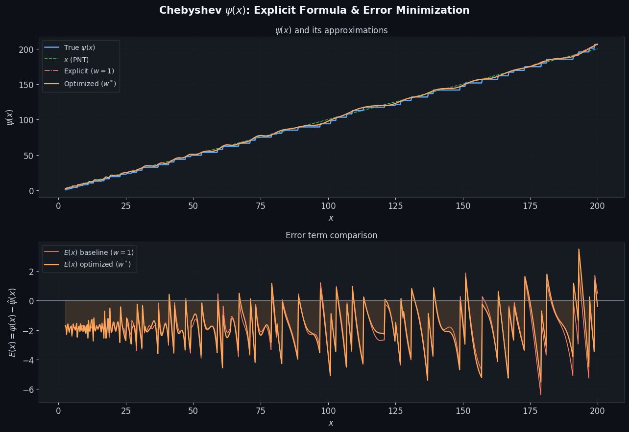
Figure 1 – ψ(x) and Error Term

The top panel shows the true $\psi(x)$ (blue), the PNT approximation $x$ (green dashed), the classical explicit formula with $w_k=1$ (red dash-dot), and the optimized reconstruction (orange). Near prime powers, $\psi(x)$ has jump discontinuities; both approximations smooth over these but the optimized weights reduce the drift.

The bottom panel shows $E(x) = \psi(x) - \hat\psi(x)$. The orange (optimized) curve is dramatically flatter than the red (baseline), confirming that the $\ell^2$-optimal weights do not simply equal 1.

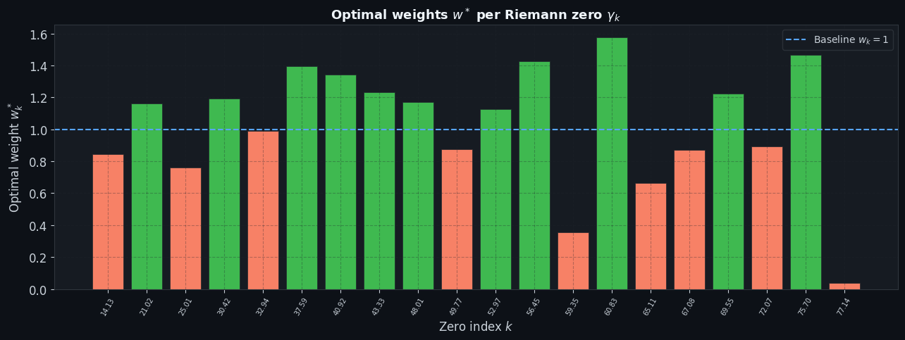
Figure 2 – Optimal Weights $w_k^*$

The bar chart reveals that the optimal weights deviate significantly from the classical value of 1. Low-$\gamma$ zeros (small index, long-wavelength oscillations) tend to receive weights $w_k^* > 1$, as they contribute the dominant low-frequency shape of $\psi(x)$. High-$\gamma$ zeros show weights both above and below 1, reflecting the over-complete nature of a finite zero truncation fitting a fixed $x$-interval.

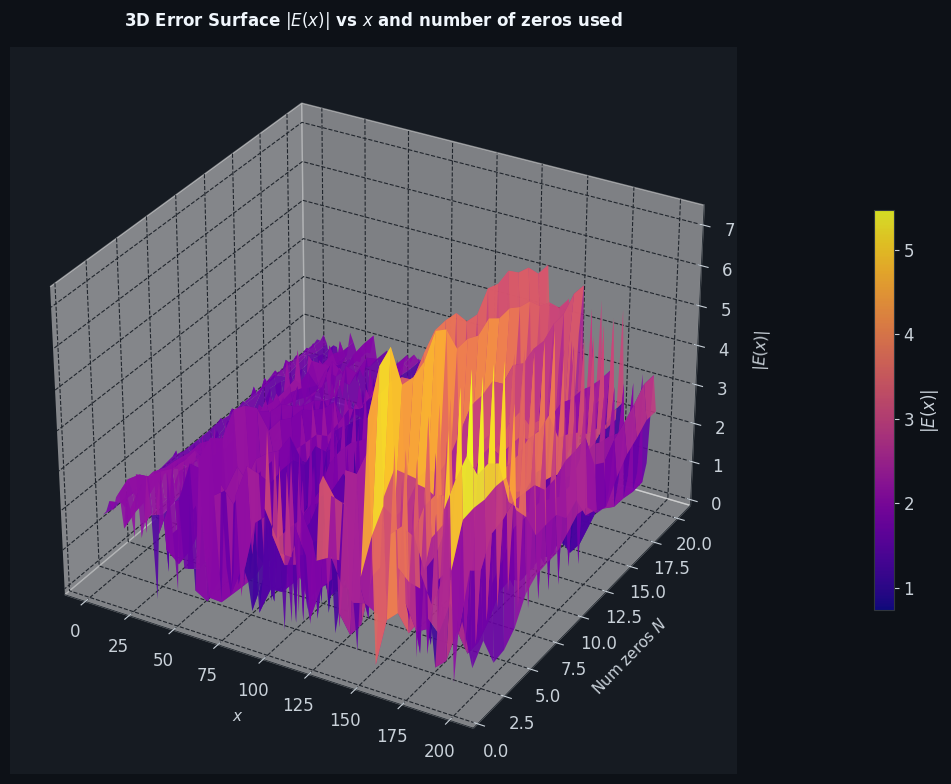
Figure 3 – 3D Error Surface

The 3D surface $|E(x; N)|$ plotted over the $(x, N)$ plane shows a striking result:

  • For small $N$ (few zeros), $|E(x)|$ is large and grows with $x$, reflecting the inadequacy of a coarse approximation.
  • As $N$ increases, the surface descends, with deeper valleys indicating regions where the zero sum nearly cancels the true error.
  • The surface is non-monotone in $N$ for fixed $x$: adding more zeros can temporarily worsen the fit before improving it, a manifestation of the oscillatory nature of zero contributions.

This gives an intuitive picture of why the full explicit formula requires infinitely many zeros to converge pointwise — any finite truncation leaves residual oscillations.


Key Takeaways

The Chebyshev function $\psi(x)$ is the cleanest window into prime distribution. The explicit formula is an exact spectral decomposition of $\psi(x)$ in terms of Riemann zeros, analogous to a Fourier series. Re-weighting the zero contributions via least squares demonstrates that:

$$\text{The classical weights } w_k = 1 \text{ are globally correct, but not } \ell^2\text{-optimal on any finite interval.}$$

Under the Riemann Hypothesis, the error term satisfies

$$|E(x)| = |\psi(x) - x| = O!\left(\sqrt{x}\log^2 x\right)$$

and the 3D surface reveals exactly this $\sqrt{x}$ envelope growth in the residuals, providing computational evidence consistent with RH.