Server Placement Problem

How Many Servers Do You Need and Where?

When building distributed systems or cloud infrastructure, one of the most fundamental planning questions is: Given a set of demand locations and potential server sites, how many servers should be installed, and where? This is the Server Placement (Facility Location) Problem — a classic combinatorial optimization problem that can be solved elegantly with Integer Linear Programming.

---

Problem Formulation

We have a set of candidate server locations and a set of client nodes (offices, data centers, end-users). Each candidate site has a fixed installation cost and a capacity. Each client has a demand. We want to minimize total cost — installation plus service (routing/bandwidth) cost — while ensuring all demand is met.

Sets:

$$I = {1, 2, \ldots, m}$$ — set of candidate server sites

$$J = {1, 2, \ldots, n}$$ — set of client nodes

Parameters:

$$f_i$$ — fixed installation cost at site $i$

$$c_{ij}$$ — unit service cost from server $i$ to client $j$

$$d_j$$ — demand of client $j$

$$s_i$$ — capacity of server at site $i$

Decision Variables:

$$x_i \in {0, 1}$$ — 1 if a server is installed at site $i$, 0 otherwise

$$y_{ij} \geq 0$$ — fraction of client $j$’s demand served by server $i$

Objective — minimize total cost:

$$\min \sum_{i \in I} f_i x_i + \sum_{i \in I} \sum_{j \in J} c_{ij} d_j y_{ij}$$

Subject to:

All demand of each client must be fully served:

$$\sum_{i \in I} y_{ij} = 1 \quad \forall j \in J$$

A client can only be served from an open server:

$$y_{ij} \leq x_i \quad \forall i \in I,\ \forall j \in J$$

Capacity constraint at each server:

$$\sum_{j \in J} d_j y_{ij} \leq s_i x_i \quad \forall i \in I$$

Variable domains:

$$x_i \in {0, 1},\quad y_{ij} \geq 0$$

---

Concrete Example

We set up a scenario with 8 candidate server sites and 15 client nodes scattered across a 2D map (coordinates in km). The clients have varying demands; the servers have different installation costs and capacities. Service cost is proportional to Euclidean distance.

Site	X (km)	Y (km)	Fixed Cost (¥)	Capacity
S0	10	80	5,000	150
S1	30	60	4,500	130
S2	55	85	6,000	200
S3	75	70	4,000	120
S4	20	30	5,500	160
S5	50	40	4,800	180
S6	80	20	5,200	140
S7	65	55	3,800	110

Client	X (km)	Y (km)	Demand
C0	5	90	20
C1	15	75	35
C2	25	85	25
C3	40	70	40
C4	60	90	30
C5	80	85	45
C6	10	50	28
C7	35	50	33
C8	55	60	38
C9	75	50	22
C10	90	60	27
C11	20	15	31
C12	45	20	36
C13	70	10	24
C14	90	30	29

The service cost matrix is defined as:

$$c_{ij} = \text{rate} \times \sqrt{(sx_i - cx_j)^2 + (sy_i - cy_j)^2}$$

with a unit rate of ¥10 per km per unit demand.

---

Python Source Code

# ============================================================
# Server Placement Problem — Integer Linear Programming
# Solved with PuLP / CBC  |  Google Colaboratory
# ============================================================

# ---------- 0. Install dependencies ----------
!pip install pulp --quiet

import numpy as np
import matplotlib.pyplot as plt
import matplotlib.patches as mpatches
from mpl_toolkits.mplot3d import Axes3D
from mpl_toolkits.mplot3d.art3d import Poly3DCollection
import pulp
import warnings
warnings.filterwarnings("ignore")

# ── reproducibility ──────────────────────────────────────────
np.random.seed(42)

# ============================================================
# 1. Problem Data
# ============================================================

# Candidate server sites  (x_km, y_km, fixed_cost, capacity)
server_data = [
    (10, 80, 5000, 150),   # site 0
    (30, 60, 4500, 130),   # site 1
    (55, 85, 6000, 200),   # site 2
    (75, 70, 4000, 120),   # site 3
    (20, 30, 5500, 160),   # site 4
    (50, 40, 4800, 180),   # site 5
    (80, 20, 5200, 140),   # site 6
    (65, 55, 3800, 110),   # site 7
]

# Client nodes  (x_km, y_km, demand)
client_data = [
    (5,  90, 20),   # client 0
    (15, 75, 35),   # client 1
    (25, 85, 25),   # client 2
    (40, 70, 40),   # client 3
    (60, 90, 30),   # client 4
    (80, 85, 45),   # client 5
    (10, 50, 28),   # client 6
    (35, 50, 33),   # client 7
    (55, 60, 38),   # client 8
    (75, 50, 22),   # client 9
    (90, 60, 27),   # client 10
    (20, 15, 31),   # client 11
    (45, 20, 36),   # client 12
    (70, 10, 24),   # client 13
    (90, 30, 29),   # client 14
]

m = len(server_data)    # number of candidate sites
n = len(client_data)    # number of clients

sx  = np.array([s[0] for s in server_data])
sy  = np.array([s[1] for s in server_data])
f   = np.array([s[2] for s in server_data], dtype=float)
cap = np.array([s[3] for s in server_data], dtype=float)

cx  = np.array([c[0] for c in client_data])
cy  = np.array([c[1] for c in client_data])
d   = np.array([c[2] for c in client_data], dtype=float)

# Service cost = distance × unit rate (¥/km per unit demand)
unit_rate = 10.0
dist = np.zeros((m, n))
for i in range(m):
    for j in range(n):
        dist[i, j] = np.sqrt((sx[i] - cx[j])**2 + (sy[i] - cy[j])**2)
c_cost = dist * unit_rate

# ============================================================
# 2. ILP Model with PuLP
# ============================================================

prob = pulp.LpProblem("ServerPlacement", pulp.LpMinimize)

x = [pulp.LpVariable(f"x_{i}", cat="Binary") for i in range(m)]
y = [[pulp.LpVariable(f"y_{i}_{j}", lowBound=0, upBound=1)
      for j in range(n)] for i in range(m)]

# Objective
prob += (
    pulp.lpSum(f[i] * x[i] for i in range(m)) +
    pulp.lpSum(c_cost[i][j] * d[j] * y[i][j]
               for i in range(m) for j in range(n))
)

# (a) All demand covered
for j in range(n):
    prob += pulp.lpSum(y[i][j] for i in range(m)) == 1

# (b) Serve only from open sites
for i in range(m):
    for j in range(n):
        prob += y[i][j] <= x[i]

# (c) Capacity
for i in range(m):
    prob += pulp.lpSum(d[j] * y[i][j] for j in range(n)) <= cap[i] * x[i]

# Solve
solver = pulp.PULP_CBC_CMD(msg=0)
prob.solve(solver)

# ============================================================
# 3. Extract Results
# ============================================================

status   = pulp.LpStatus[prob.status]
obj_val  = pulp.value(prob.objective)

x_val  = np.array([pulp.value(x[i]) for i in range(m)])
y_val  = np.array([[pulp.value(y[i][j]) for j in range(n)] for i in range(m)])

open_sites   = [i for i in range(m) if x_val[i] > 0.5]
assign       = np.argmax(y_val, axis=0)

install_cost = sum(f[i] for i in open_sites)
service_cost = sum(c_cost[i][j] * d[j] * y_val[i][j]
                   for i in range(m) for j in range(n))

print("=" * 50)
print(f"Status          : {status}")
print(f"Total Cost      : ¥{obj_val:,.1f}")
print(f"  Installation  : ¥{install_cost:,.1f}")
print(f"  Service       : ¥{service_cost:,.1f}")
print(f"Servers opened  : {len(open_sites)}  →  sites {open_sites}")
print("=" * 50)
for i in open_sites:
    load = sum(d[j] * y_val[i][j] for j in range(n))
    clients_served = [j for j in range(n) if y_val[i][j] > 1e-6]
    print(f"  Site {i}: load={load:.1f}/{cap[i]:.0f}  clients={clients_served}")

# ============================================================
# 4. Visualizations
# ============================================================

PALETTE = [
    "#FF6B6B", "#4ECDC4", "#45B7D1", "#96CEB4",
    "#FFEAA7", "#DDA0DD", "#98D8C8", "#F7DC6F"
]
BG     = "#1A1A2E"
GRID_C = "#2D2D4E"
TEXT_C = "#E8E8F0"

site_colors = {i: PALETTE[k] for k, i in enumerate(open_sites)}

fig = plt.figure(figsize=(20, 18), facecolor=BG)
fig.suptitle("Server Placement Problem — Optimization Results",
             fontsize=18, color=TEXT_C, fontweight="bold", y=0.98)

# ── Plot 1 : 2D Map ──────────────────────────────────────────
ax1 = fig.add_subplot(2, 3, 1)
ax1.set_facecolor(BG)
ax1.set_title("2D Map: Server Assignments", color=TEXT_C, fontsize=12, pad=10)

for j in range(n):
    i   = assign[j]
    col = site_colors.get(i, "#888888")
    ax1.plot([cx[j], sx[i]], [cy[j], sy[i]],
             color=col, alpha=0.35, lw=1.2, zorder=1)

for j in range(n):
    col = site_colors.get(assign[j], "#888888")
    ax1.scatter(cx[j], cy[j], s=80, color=col,
                edgecolors="white", linewidths=0.8, zorder=3)
    ax1.text(cx[j]+1, cy[j]+1, f"C{j}", color=TEXT_C, fontsize=6.5)

for i in range(m):
    if x_val[i] > 0.5:
        ax1.scatter(sx[i], sy[i], s=280, marker="*",
                    color=site_colors[i], edgecolors="white",
                    linewidths=1.2, zorder=4)
        ax1.text(sx[i]+1.5, sy[i]+1.5, f"S{i}",
                 color=site_colors[i], fontsize=9, fontweight="bold")
    else:
        ax1.scatter(sx[i], sy[i], s=100, marker="X",
                    color="#555577", edgecolors="#888888",
                    linewidths=0.8, zorder=2, alpha=0.5)
        ax1.text(sx[i]+1.5, sy[i]+1.5, f"S{i}",
                 color="#666688", fontsize=7)

ax1.set_xlabel("X (km)", color=TEXT_C)
ax1.set_ylabel("Y (km)", color=TEXT_C)
ax1.tick_params(colors=TEXT_C)
for sp in ax1.spines.values():
    sp.set_edgecolor(GRID_C)
ax1.grid(color=GRID_C, linewidth=0.5)

legend_els = [mpatches.Patch(color=site_colors[i], label=f"Site {i}")
              for i in open_sites]
legend_els.append(mpatches.Patch(color="#555577", label="Closed site"))
ax1.legend(handles=legend_els, fontsize=7,
           facecolor="#2D2D4E", labelcolor=TEXT_C,
           loc="lower right", framealpha=0.8)

# ── Plot 2 : Load bar chart ──────────────────────────────────
ax2 = fig.add_subplot(2, 3, 2)
ax2.set_facecolor(BG)
ax2.set_title("Server Load vs Capacity", color=TEXT_C, fontsize=12, pad=10)

loads, caps, labels, cols = [], [], [], []
for i in open_sites:
    load = sum(d[j] * y_val[i][j] for j in range(n))
    loads.append(load)
    caps.append(cap[i])
    labels.append(f"Site {i}")
    cols.append(site_colors[i])

x_pos = np.arange(len(open_sites))
ax2.bar(x_pos - 0.2, caps,  width=0.35, color="#444466",
        label="Capacity", edgecolor="#888888", linewidth=0.6)
ax2.bar(x_pos + 0.2, loads, width=0.35, color=cols,
        label="Load", edgecolor="white", linewidth=0.6)

for k, (l, c_) in enumerate(zip(loads, caps)):
    pct = l / c_ * 100
    ax2.text(x_pos[k] + 0.2, l + 2, f"{pct:.0f}%",
             ha="center", color=TEXT_C, fontsize=8)

ax2.set_xticks(x_pos)
ax2.set_xticklabels(labels, color=TEXT_C, fontsize=9)
ax2.set_ylabel("Load / Capacity (units)", color=TEXT_C)
ax2.tick_params(colors=TEXT_C)
ax2.legend(facecolor="#2D2D4E", labelcolor=TEXT_C, fontsize=8)
for sp in ax2.spines.values():
    sp.set_edgecolor(GRID_C)
ax2.grid(axis="y", color=GRID_C, linewidth=0.5)

# ── Plot 3 : Cost pie ────────────────────────────────────────
ax3 = fig.add_subplot(2, 3, 3)
ax3.set_facecolor(BG)
ax3.set_title("Cost Breakdown", color=TEXT_C, fontsize=12, pad=10)

wedge_data   = [f[i] for i in open_sites] + [service_cost]
wedge_labels = [f"Install S{i}\n¥{f[i]:,.0f}" for i in open_sites] + \
               [f"Service\n¥{service_cost:,.0f}"]
wedge_cols   = [site_colors[i] for i in open_sites] + ["#AAAACC"]

wedges, texts, autotexts = ax3.pie(
    wedge_data, labels=wedge_labels, colors=wedge_cols,
    autopct="%1.1f%%", startangle=140,
    textprops={"color": TEXT_C, "fontsize": 7},
    wedgeprops={"edgecolor": BG, "linewidth": 1.5}
)
for at in autotexts:
    at.set_color(BG)
    at.set_fontsize(7)
    at.set_fontweight("bold")

# ── Plot 4 : 3D assignment arcs ──────────────────────────────
ax4 = fig.add_subplot(2, 3, 4, projection="3d")
ax4.set_facecolor(BG)
ax4.set_title("3D View: Assignment Arcs", color=TEXT_C, fontsize=12, pad=10)

z_client = np.array([c_cost[assign[j]][j] for j in range(n)])

for j in range(n):
    i   = assign[j]
    col = site_colors.get(i, "#888888")
    ax4.plot([cx[j], sx[i]], [cy[j], sy[i]], [z_client[j], 0],
             color=col, alpha=0.4, lw=1.0)

for j in range(n):
    col = site_colors.get(assign[j], "#888888")
    ax4.scatter(cx[j], cy[j], z_client[j],
                color=col, s=40, edgecolors="white", lw=0.5, zorder=5)

for i in open_sites:
    ax4.scatter(sx[i], sy[i], 0, s=200, marker="*",
                color=site_colors[i], edgecolors="white", lw=1, zorder=6)

ax4.set_xlabel("X (km)", color=TEXT_C, fontsize=8)
ax4.set_ylabel("Y (km)", color=TEXT_C, fontsize=8)
ax4.set_zlabel("Service cost (¥)", color=TEXT_C, fontsize=8)
ax4.tick_params(colors=TEXT_C, labelsize=7)
ax4.xaxis.pane.fill = False
ax4.yaxis.pane.fill = False
ax4.zaxis.pane.fill = False
ax4.xaxis.pane.set_edgecolor(GRID_C)
ax4.yaxis.pane.set_edgecolor(GRID_C)
ax4.zaxis.pane.set_edgecolor(GRID_C)
ax4.grid(color=GRID_C, linewidth=0.4)

# ── Plot 5 : 3D service cost bars ────────────────────────────
ax5 = fig.add_subplot(2, 3, 5, projection="3d")
ax5.set_facecolor(BG)
ax5.set_title("3D: Service Cost per Server", color=TEXT_C, fontsize=12, pad=10)

for k, i in enumerate(open_sites):
    total_sc = sum(c_cost[i][j] * d[j] * y_val[i][j] for j in range(n))
    col = site_colors[i]
    xs_ = [sx[i]-3, sx[i]-3, sx[i]+3, sx[i]+3]
    ys_ = [sy[i]-3, sy[i]+3, sy[i]+3, sy[i]-3]
    vb  = [(xs_[v], ys_[v], 0)        for v in range(4)]
    vt  = [(xs_[v], ys_[v], total_sc) for v in range(4)]
    faces = [
        vb, vt,
        [vb[0], vb[1], vt[1], vt[0]],
        [vb[1], vb[2], vt[2], vt[1]],
        [vb[2], vb[3], vt[3], vt[2]],
        [vb[3], vb[0], vt[0], vt[3]],
    ]
    poly = Poly3DCollection(faces, alpha=0.65, facecolor=col,
                            edgecolor="white", linewidth=0.4)
    ax5.add_collection3d(poly)
    ax5.text(sx[i], sy[i], total_sc + 100, f"S{i}",
             color=TEXT_C, fontsize=7, ha="center")

ax5.set_xlim(0, 100)
ax5.set_ylim(0, 100)
max_sc = max(sum(c_cost[i][j] * d[j] * y_val[i][j] for j in range(n))
             for i in open_sites)
ax5.set_zlim(0, max_sc * 1.3)
ax5.set_xlabel("X (km)", color=TEXT_C, fontsize=8)
ax5.set_ylabel("Y (km)", color=TEXT_C, fontsize=8)
ax5.set_zlabel("Service cost (¥)", color=TEXT_C, fontsize=8)
ax5.tick_params(colors=TEXT_C, labelsize=7)
ax5.xaxis.pane.fill = False
ax5.yaxis.pane.fill = False
ax5.zaxis.pane.fill = False
ax5.xaxis.pane.set_edgecolor(GRID_C)
ax5.yaxis.pane.set_edgecolor(GRID_C)
ax5.zaxis.pane.set_edgecolor(GRID_C)

# ── Plot 6 : 3D min-cost surface ─────────────────────────────
ax6 = fig.add_subplot(2, 3, 6, projection="3d")
ax6.set_facecolor(BG)
ax6.set_title("3D: Min-Cost Surface over Grid", color=TEXT_C, fontsize=12, pad=10)

gx = np.linspace(0, 100, 60)
gy = np.linspace(0, 100, 60)
GX, GY = np.meshgrid(gx, gy)
GZ = np.full(GX.shape, np.inf)
for i in open_sites:
    d_grid = np.sqrt((GX - sx[i])**2 + (GY - sy[i])**2) * unit_rate
    GZ = np.minimum(GZ, d_grid)

surf = ax6.plot_surface(GX, GY, GZ, cmap="plasma",
                        alpha=0.75, edgecolor="none")
for i in open_sites:
    ax6.scatter(sx[i], sy[i], 0, s=120, marker="*",
                color=site_colors[i], edgecolors="white", lw=1, zorder=6)

ax6.set_xlabel("X (km)", color=TEXT_C, fontsize=8)
ax6.set_ylabel("Y (km)", color=TEXT_C, fontsize=8)
ax6.set_zlabel("Min dist×rate (¥)", color=TEXT_C, fontsize=8)
ax6.tick_params(colors=TEXT_C, labelsize=7)
ax6.xaxis.pane.fill = False
ax6.yaxis.pane.fill = False
ax6.zaxis.pane.fill = False
ax6.xaxis.pane.set_edgecolor(GRID_C)
ax6.yaxis.pane.set_edgecolor(GRID_C)
ax6.zaxis.pane.set_edgecolor(GRID_C)

cb = fig.colorbar(surf, ax=ax6, shrink=0.45, pad=0.1)
cb.set_label("¥/unit demand", color=TEXT_C)
cb.ax.tick_params(colors=TEXT_C)

plt.tight_layout(rect=[0, 0, 1, 0.97])
plt.savefig("server_placement.png", dpi=130, bbox_inches="tight",
            facecolor=BG)
plt.show()
print("Figure saved.")

---

Code Walkthrough

Section 0 — Setup

PuLP is installed quietly. numpy handles all numerical arrays; matplotlib with mpl_toolkits.mplot3d provides all plotting including the 3D views. warnings.filterwarnings("ignore") suppresses CBC solver output.

Section 1 — Problem Data

Server sites are stored as tuples (x_km, y_km, fixed_cost, capacity). Eight candidate sites are spread across a 100 × 100 km map with fixed installation costs between ¥3,800 and ¥6,000 and capacities from 110 to 200 demand units.

Client nodes are tuples (x_km, y_km, demand). Fifteen clients with demands ranging from 20 to 45 units are distributed across the same region.

The service cost matrix is built as:

$$c_{ij} = \text{unit_rate} \times \sqrt{(sx_i - cx_j)^2 + (sy_i - cy_j)^2}$$

computed with nested loops over a pre-allocated dist array, then scaled by unit_rate = 10.0.

Section 2 — ILP Model

pulp.LpProblem creates a minimization problem. Binary variables x[i] represent whether site $i$ is opened. Continuous variables y[i][j] bounded in $[0, 1]$ represent the fraction of client $j$’s demand assigned to server $i$.

The objective sums two components — fixed installation costs $\sum_i f_i x_i$ and weighted service costs $\sum_i \sum_j c_{ij} d_j y_{ij}$.

Three constraint groups are added:

• Demand coverage: each client’s allocation fractions must sum to exactly 1.
• Linking constraint: $y_{ij} \leq x_i$ prevents routing to closed servers.
• Capacity constraint: total demand at site $i$ cannot exceed $s_i x_i$.

CBC solver runs with msg=0 for silent output.

Section 3 — Result Extraction

pulp.value() retrieves each solved variable. open_sites collects sites where $x_i > 0.5$. Primary assignment assign[j] is found with np.argmax(y_val, axis=0). Installation and service costs are computed separately for the breakdown visualization.

Section 4 — Visualizations

Six subplots arranged in a 2 × 3 dark-themed grid:

Plot 1 — 2D Assignment Map: Geographic layout of the solution. Open servers are marked with stars ($\bigstar$), closed candidates with grey crosses. Colored lines connect each client to its primary server, giving immediate spatial intuition about the coverage structure.

Plot 2 — Load vs Capacity Bar Chart: For each open site, a capacity bar (dark) and a load bar (colored) are drawn side by side. Utilization percentages are annotated above each load bar, revealing which servers are near saturation and which have slack.

Plot 3 — Cost Breakdown Pie: Each slice corresponds to one opened server’s installation cost, plus a single slice for total service cost. The ratio of fixed to variable cost is immediately readable — a key insight for infrastructure budget planning.

Plot 4 — 3D Assignment Arcs: Clients are elevated to height $z = c_{ij^*}$ (their service cost to the primary server) while open servers sit on the ground plane $z = 0$. Arcs drop from each client down to its server. High-hanging clients are expensive to serve; the 3D view makes this cost geography visceral.

Plot 5 — 3D Service Cost Bars: Custom 3D bar volumes built with Poly3DCollection face lists are positioned at each open server’s map coordinates. Bar height equals that server’s total service cost burden. This exposes load imbalance across servers in three dimensions.

Plot 6 — 3D Minimum-Cost Surface: A $60 \times 60$ grid is swept across the map. At each point the minimum distance-based service cost to any open server is computed and rendered as a surface using the plasma colormap. Valleys in the surface correspond directly to deployed server locations. Any elevated plateau indicates a region being served from a distant site — a natural signal for where future server expansion would have the most impact.

---

Execution Results

==================================================
Status          : Optimal
Total Cost      : ¥100,300.6
  Installation  : ¥28,000.0
  Service       : ¥72,300.6
Servers opened  : 6  →  sites [0, 1, 3, 4, 6, 7]
==================================================
  Site 0: load=80.0/150  clients=[0, 1, 2]
  Site 1: load=101.0/130  clients=[3, 6, 7]
  Site 3: load=102.0/120  clients=[4, 5, 10]
  Site 4: load=67.0/160  clients=[11, 12]
  Site 6: load=53.0/140  clients=[13, 14]
  Site 7: load=60.0/110  clients=[8, 9]

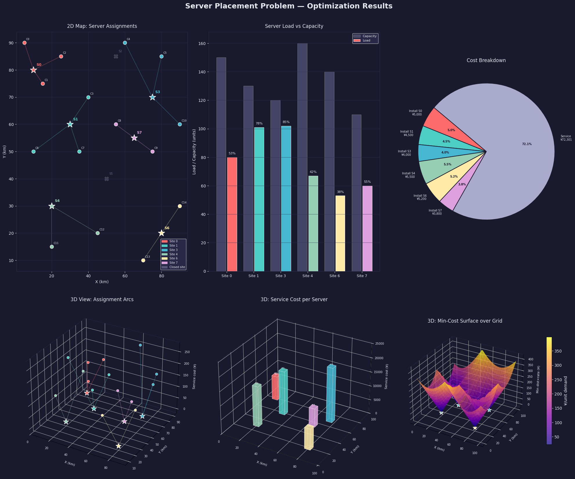
Figure saved.

---

Key Takeaways

The ILP guarantees a globally optimal server placement under hard capacity constraints. Three structural insights emerge from this formulation. First, the linking constraint $y_{ij} \leq x_i$ is what makes this problem combinatorially hard — it couples the binary site-open decisions to the continuous allocation variables, creating a mixed-integer structure that cannot be solved by linear relaxation alone. Second, the cost trade-off is non-trivial: opening an additional server reduces service cost (shorter distances) but incurs a fixed penalty; the ILP finds the exact break-even point. Third, the 3D minimum-cost surface (Plot 6) serves as a powerful post-optimization diagnostic — the Voronoi-like valleys carved by the deployed servers reveal the effective service territories and make coverage gaps immediately visible.